Fundamental Photogrammetry Algorithms

Photogrammetry

This repository holds my experiments about fundamental tasks in photogrammetry

• Basic Homography Math
• Panorama
• Camera calibration
• Epipolar Constraint
• Triangulation
• Dense Stereo Correspondence

Basic Homography Math

This code consists of basic transformations on the homography representations of line and point

Panorama

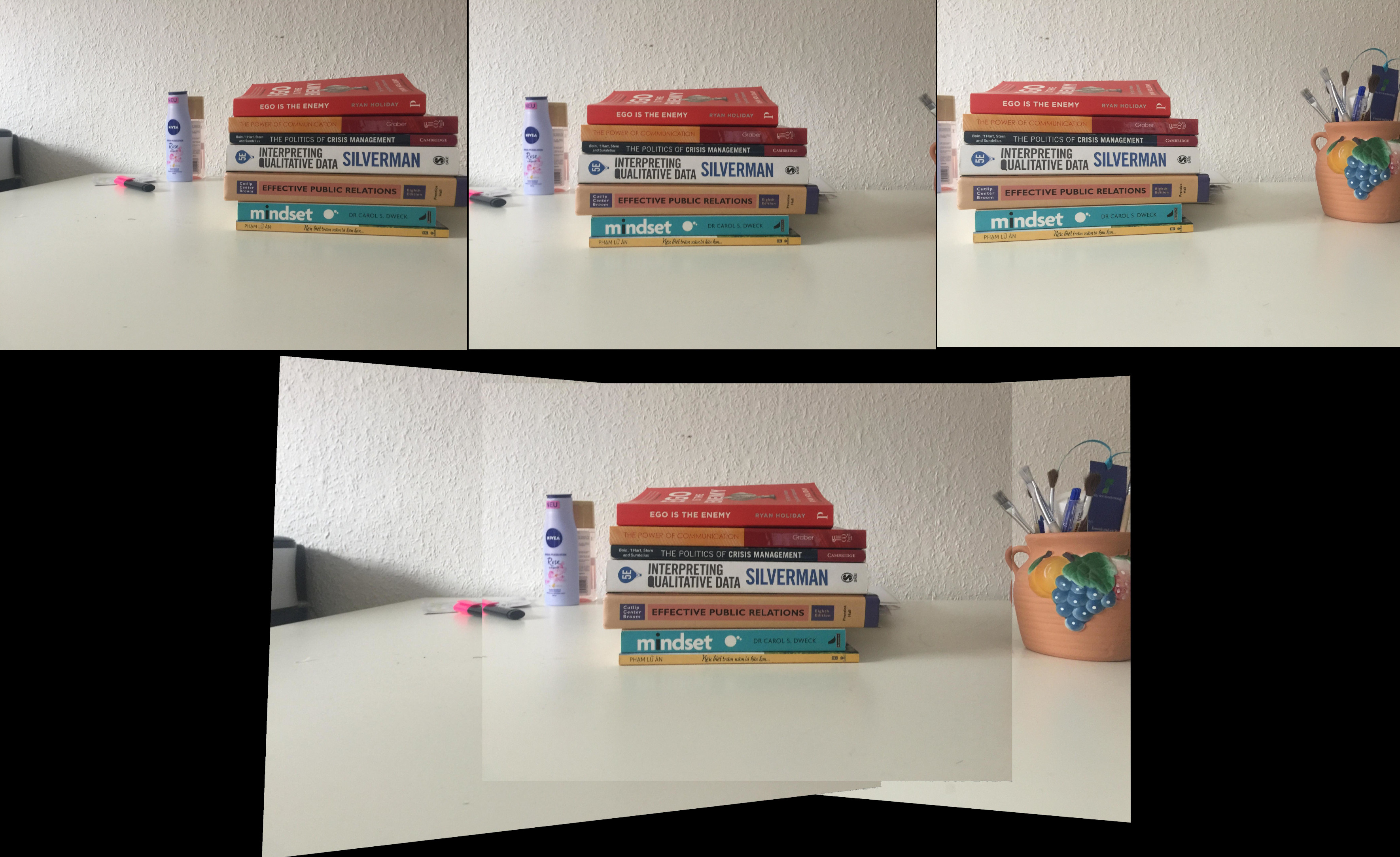
In this experiment, I stitched 3 pictures of a subject into a single panorama picture.The experiment includes the following steps

• 3 input pictures are taken by turning camera around a common projection center so that three images do not have disparity
• Correspondence analysis is performed by selecting feature points in 3 images in a way that they are both on common planar surface. These feature points will be used to estimate homography transformations from one image to another image. The homography is estimated using SVD.
• Finally, image one is rectified to the plane of the image 2, and then the rectified image 2-3 is one more time rectified to the plane of the image 3.

Camera calibration

This experiment is about camera calibration using direct linear transformation (DLT), which estimate the intrinsic and extrinsic camera parameters using correspondences between 3D-2D control points. The experiment include the following stages.

• Correspondence analysis: the 2D control points on image are selected manually using a Matlab tool. The corresponding 3D control points are generated in code based on the pattern that we draw on the calibration object. At least 6 point correspondences are required for the DLT algorithm.
• The projective transformation is then estimated from the correspondence points using SVD decomposition.
• In the final stage, the estimated projection is decomposed using RQ decomposition. The result of RQ decomposition include two matrices: a 3x3 matrix that represents the intrinsic parameters and a 3x4 matrix that represents the extrinsic camera parameters (rotation and translation)

Epipolar Constraint

• In a pair of stereo images, 3D points are projected onto two corresponding points on the left and right images. The relation between these tie points are encoded in the $3\times3$ fundamental matrix $F$, which represent the relations between left points $x$ and right points $x’$ through the equation $x’^TFx$. However, due to the fact that the rank of the fundamental is just 2, it just maps one point on the left to the corresponding line on the image, as shown in the below figure.

• in this experiment, I tried to visualize the epipolar contraint on feature points through the following steps:
  • select corresponding feature points on two stereo images
  • estimate the fundamental matrix
  • using the fundamental matrix to transform each feature point into the corresponding epipolar line on the other image. The visualizaiont of these lines are shown in the below figure.

  

Triangulation

In this experiment, the 3D point cloud of a subject is reconstructed from a set of tie points in the two stereo images. The algorithm includes the two main stages

• Projective reconstruction
  • First the fundamental matrix between the two stereo images are estimated using feature points.

  • From the fundamental matrix, we create a pair of perspective projection matrices for two images. There is an unlimited number of projection matrices that could be created from the fundamental matrix, but we just pick one.

  • we create a linear equation that relate 3D points to corresponding image points through the projection matrix. Solving this equation gives us 3D points in the projective space, which is shown in the below figure
• Euclidean reconstruction After the previous step, our point cloud is still in the projective space, which looks distorted. To make it look as what we often see everyday, we need to estimate a 3D homography that will transforms the projective point cloud to the Euclidean space.
  • Given at least 5.5 3D control points we create a linear equation that relate projective points to corresponding 3D control points. Solving this equation will give us the 3D homography.
  • We then apply the homography to transform our projective point cloud to Euclidean space. The final point is shown in the below.

Dense Stereo Correspondence

In this experiment, the disparity map is calculated from a pair of rectified stereo image. Rectified means that two input images are transformed by a planar homography in a way that two camera plane are parallel to each other, which is often a normal stereo rig. The rectified images bring us two advantages

• First the correspondence analysis could be reduced to a 1D search problem. Given a point in the left image, its corresponding point in the second image could be found by searching along the same row. After the corresponding point is found, the disparity value is calculated as the shift between two points along the horizontal axis.
• Secondly, in the normal case, the depth value is inversely proportional to the disparity value, which means that we could directly calculate the depth map if we know the disparity map.

Below is a visualize of the disparity map. We can can see that the closer a point to the camera, the lighter the corresponding pixel is. This show that the disparity is inversely proportional to the depth value

Contact

if you have further question about the code, you can contact me through my email khanhhh89@gmail.com