Thin Plate Splines Warping
- Introduction
- What is an image warping problem?
- Image Warping Applications
- Thin Plate Spline
- OpenCV Thin Plate Spline implementation
- Conclusion
- References
Introduction
I have been using the Thin Plate Warping algorithm from OpenCV for quite a long time, but still, just have a vague idea about it. It often makes me feel uncomfortable. Therefore, I set out to read the paper about Thin Plate Warping and dig deep into the OpenCV implementation to get a better insight into the method. This article is the summary I wrote along my journey, as a way to reorganize concepts. Hopefully, it would be useful for you as it was to me.
What is an image warping problem?
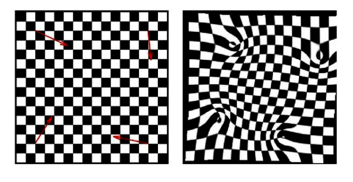
Given an image with a sparse set of control points $(x_i, y_i)$ with corresponding displacements $(\Delta{x_i}, \Delta{y_i})$ , we want to find a mapping $f: (x,y) \to (x’, y’)$ from pixels in the input image to pixels in the warped/deformed image so that the corresponding warped control points $(x’_i, y’_i)$ closely match its expected targets $(x_i + \Delta{x_i}, y_i + \Delta{y_i})$, and the surrounding points are deformed as smoothly as possible.
As depicted in the below figure, the red arrows represent $4$ point correspondences between the left and the right image. The origin of red arrows represent control points $(x_i,y_i)$ in the left image, and the end of the arrows represent the corresponding control points $(x_i+\Delta{x_i}, y_i+\Delta{y_i})$ in the right image, but plotted in the left image. Given this information, we want to find a smooth interpolation function or a warping field that maps all 2D points from the left image to the right image. The result of the warping algorithm will look like the right image in below.
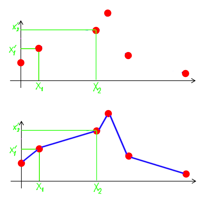
In the 1-dimensional space, this problem could be stated that given a sparse set of correspondences $(x_i, x’_i)$ as shown by red points, we want to estimate a smooth function that maps every points $x$ to $x’$.
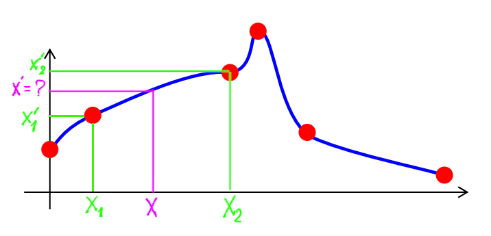
Image Warping Applications
Several applications of image warping are shown in below.
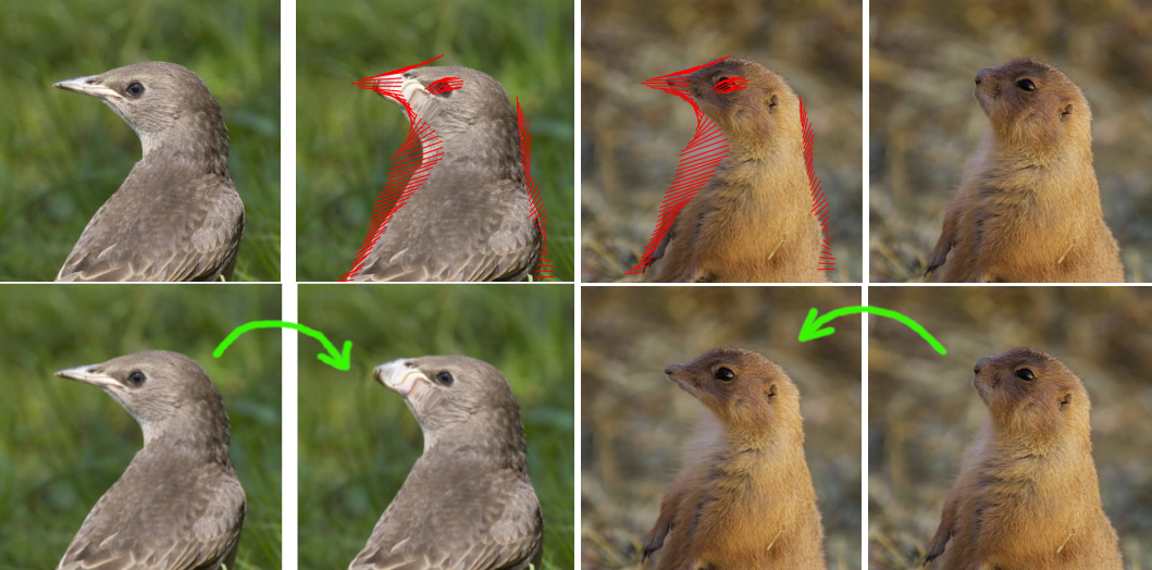
Image editing
Given a contour of a subject, artists might want to warp/deform the subject in some way by moving control points along the contour
Texture mapping
Given two sets of facial landmarks in the input image and the texture space, we can warp the input image to the texture so that it could be displayed in 3D.
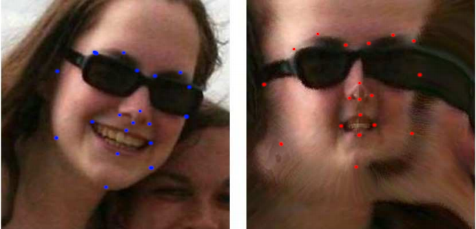
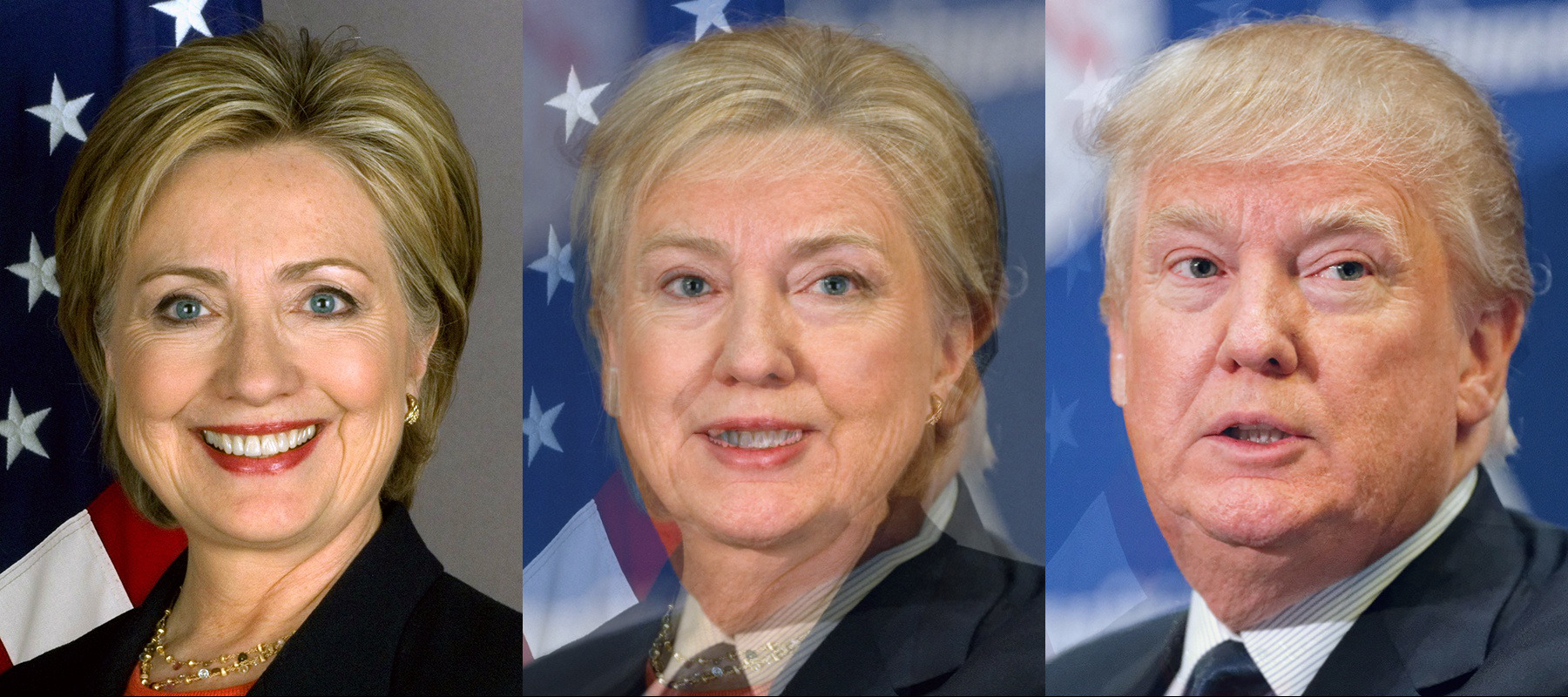
Image morphing
Given two sets of facial landmarks in two images, one face could be warped to make it look like the other face.
Radial Basis Function interpolation
Before introducing the Thin Plate Spline warping algorithm, we will quickly go through the radial basis function interpolation, which is the general form of the thin plate spline interpolation problem. We will just focus on explaining the $1D$ example introduced in the last section.
In the beginning, the only information we have is a sparse set of control point correspondences. The most simple way to infer the other points is a linear interpolation, where interpolated points will move along the segment connecting the two closest control points, as shown below.
However, what we want is a smooth interpolation function that goes through control points closely. This is the place that the Radial Basis Function comes to help. As explained in this lecture note, Radial basis functions are smooth kernels centered around control points $x_i$. The further an interpolated point $x$ from a control point $x_i$, the smaller its distance to the corresponding kernel and therefore, the less it is affected by the kernel. Some kernels, due to the larger density of its neighboring points around its center and its size, could have a larger influence on the whole smooth contour than other kernels.
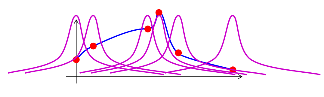
In general, instead of interpolating from just two closest points as in our above linear interpolation example, with radial basis function, each point will be calculated a weighted combination of all kernel distances, as summarized by the following function. Given an input point $x$, this smooth interpolation function will return the corresponding warped point $x’ = f(x)$
where $\alpha_i$ is the weight corresponding to the radial basis function $R(x,x_i)$ around the point $x_i$
$\alpha_i$ is found as the solution to a linear system formed by setting $f(x)$ to $f(x_i)$ for all control points $x_i$. For example, if we have 3 control point correspondences $(x_0, x’_0)$, $(x_1, x’_1)$, $(x_2, x’_2)$, the corresponding weights $\alpha_0$, $\alpha_1$, $\alpha_2$ will be the solution to the following linear system
The solution to the system will be
The possible radial basis functions could be a gaussian kernel $e^{\frac{-r^2}{2\sigma}}$ or $r^2 log(r)$, which is the thin-plate-spline function for the $1D$ case.
Thin Plate Spline
Now we will explain the Thin Plate Spline warping algorithm for our 2D warping problem.
What to solve for?
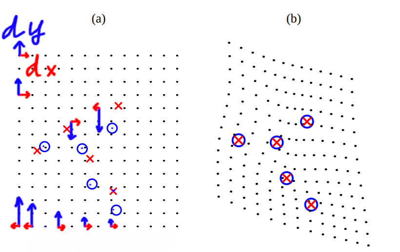
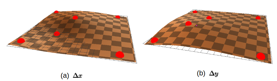
In the below figures, we refine a bit further the definition of the thin plate spline warping problem. Given red cross points the input images that are expected to move to blue circle points, we want to solve for two smooth functions from which we can sample for discrete displacements along $x$ and $y$ directions, as depicted by the red and blue arrows in the below figure.
The two smooth functions are shown below, as modified from the original equations in the paper
These two functions give us the warped points $(x’, y’)$ given origin grid points $(x_i, y_i)$ in the left input image. The two below figure visualize $\Delta_x$ and $\Delta_y$ displacements between $(x’_i, y’_i)$ and $(x_i, y_i)$ as the height of a 3D smooth.
As explained in the article by hlombaert,
The three first coefficients $(a_1, a_x, a_y)$ represents the linear plane that best approximates all $x’$ (or $y’$) of all control points $(x_i, y_i)$.
The later terms $w_i$ for $i \in [0,N)$ denotes the weight of its kernel surrounding each control point to the final $x$ or $y$ displacement.
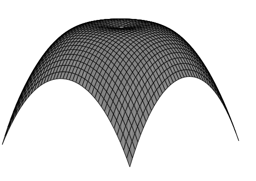
The terms
represents the distance from a control point $(x_j,y_j)$ to the kernel of the control point $(x_i, y_i)$. The visualization of this thin plate spline kernel $U(r) = r^2log(r)$ is shown in below. The closer a point to the kernel center (a control point), the higher its height or the return value is.
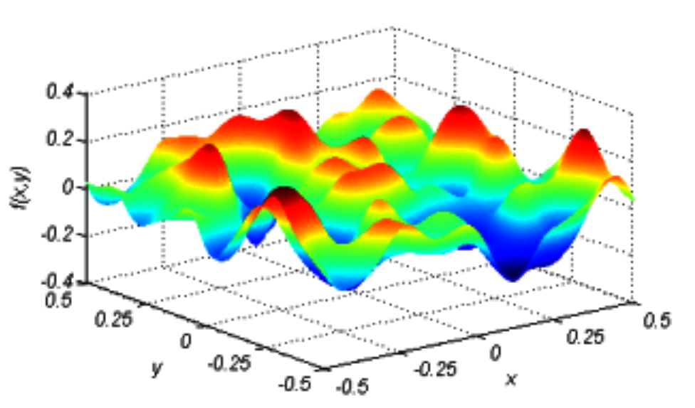
The below visualization of a complex surface could be used to imagine how all the kernels look like when they are multiplied by their corresponding weights $w_i$
How to solve
Coefficients $(a, a_x, a_y, w_i)$ of each thin plate spline function are found by solving the following linear system
where $ K_{ij} = U(distance((x_i,y_i), (x_j, y_j)) $ , the ith of P is $(1, x_i, y_i)$.
The top row of the left side $[K \ \ P]$ $\times$ $[v, o]^T$ represents the function $f_{x’}$ or $f_{y’}$ with all control points $(x_i, y_i)$ substituted.
The second row $[P^T\ \ O]$ represents additional constraints to the system, as explained in the section C in the paper.
To make it clear, we will build a linear system to solve for coefficients of $f_{x’i}$ and $f{y’_i}$ given 3 control point correspondences.
The linear system for the TPS function $f_{x’} $ will look like as follows.
and the TPS function $f_{y’}$
OpenCV Thin Plate Spline implementation
In this part, I will explain how the theoretical stages we discussed so far are realized in the OpenCV implementation.
The Thin Plate Spline Kernel function
Below is the kernel function that calculates the distance from a point $p$ to a kernel represented by the point $q$. The input $r$ to the equation is the squared distance to the kernel center.
static float distance(Point2f p, Point2f q)
{
    Point2f diff = p - q;
    float norma = diff.x*diff.x + diff.y*diff.y;// - 2*diff.x*diff.y;
    if (norma<0) norma=0;
    //else norma = std::sqrt(norma);
    norma = norma*std::log(norma+FLT_EPSILON);
    return norma;
}
Build matrix L
The matrix L is built from the input control point set in the input image. It consists of 3 main blocks:
- K: distance between control point and kernels, calculated by the function distance above.
- P: the input control points: $(1, x_i, y_i)$
- O: zero block representing constraints on $w_i$ and $x_i$, $y_i$.
// Building the matrices for solving the L*(w|a)=(v|0) problem with L={[K|P];[P'|0]}
// Building K and P (Needed to build L)
Mat matK((int)matches.size(),(int)matches.size(),CV_32F);
Mat matP((int)matches.size(),3,CV_32F);
for (int i=0, end=(int)matches.size(); i<end; i++)
{
    for (int j=0; j<end; j++)
    {
        if (i==j)
        {
            // in our setting, it K[i,i] = 0, but here opencv add regulerization factor
            matK.at<float>(i,j)=float(regularizationParameter);
        }
        else
        {
            // calculate distance from point j to the TSP kernel i
            matK.at<float>(i,j) = distance(Point2f(shape1.at<float>(i,0),shape1.at<float>(i,1)),
                                           Point2f(shape1.at<float>(j,0),shape1.at<float>(j,1)));
        }
    }

    // set point (x_i, y_i) to the matrix P
    matP.at<float>(i,0) = 1;
    matP.at<float>(i,1) = shape1.at<float>(i,0);
    matP.at<float>(i,2) = shape1.at<float>(i,1);
}

// Building L
// Copy K, P, P^T blocks to the matrix L
Mat matL=Mat::zeros((int)matches.size()+3,(int)matches.size()+3,CV_32F);
Mat matLroi(matL, Rect(0,0,(int)matches.size(),(int)matches.size())); //roi for K
matK.copyTo(matLroi);
matLroi = Mat(matL,Rect((int)matches.size(),0,3,(int)matches.size())); //roi for P
matP.copyTo(matLroi);
Mat matPt;
transpose(matP,matPt);
matLroi = Mat(matL,Rect(0,(int)matches.size(),(int)matches.size(),3)); //roi for P'
matPt.copyTo(matLroi);
Build the right hand side $[v\ o]^T$
the right hand side is built from target control points $x’_i$ and $y’_i$
//Building B (v|0)
Mat matB = Mat::zeros((int)matches.size()+3,2,CV_32F);
for (int i=0, end = (int)matches.size(); i<end; i++)
{
    matB.at<float>(i,0) = shape2.at<float>(i,0); //x's
    matB.at<float>(i,1) = shape2.at<float>(i,1); //y's
}
Solve for $f_{x’}$ and $f_{x’}$
//Obtaining transformation params (w|a)
solve(matL, matB, tpsParameters, DECOMP_LU);
//tpsParameters = matL.inv()*matB;

//Setting transform Cost and Shape reference
Mat w(tpsParameters, Rect(0,0,2,tpsParameters.rows-3));
Mat Q=w.t()*matK*w;
transformCost=fabs(Q.at<float>(0,0)*Q.at<float>(1,1));//fabs(mean(Q.diag(0))[0]);//std::max(Q.at<float>(0,0),Q.at<float>(1,1));
tpsComputed=true;
Warp image using estimated $f_{x’}$ and $f_{y’}$
In this part, the main stages to warp a real input image from the estimated Thin-Plate function in the previous section will be described in detail.
Build remap data structure
First a remap data structure will be constructed by sampling from the estimated continuous functions $f_{x_i’}$, and $f_{y_i’}$. This data structure stores warped/deformed locations in the warped image for each location in the input image. An OpenCV function called remap will use this data to interpolate colors for every pixel in the warped image.
/* public methods */
void ThinPlateSplineShapeTransformerImpl::warpImage(InputArray transformingImage, OutputArray output, int flags, int borderMode, const Scalar& borderValue) const
{
    CV_INSTRUMENT_REGION();

    CV_Assert(tpsComputed==true);

    Mat theinput = transformingImage.getMat();
    Mat mapX(theinput.rows, theinput.cols, CV_32FC1);
    Mat mapY(theinput.rows, theinput.cols, CV_32FC1);

    // for each pixel in the input image
    for (int row = 0; row < theinput.rows; row++)
    {
        // for each pixel in the input image
        for (int col = 0; col < theinput.cols; col++)
        {
            // sample the corresponding location in the warped image space
            Point2f pt = _applyTransformation(shapeReference, Point2f(float(col), float(row)), tpsParameters);
            mapX.at<float>(row, col) = pt.x;
            mapY.at<float>(row, col) = pt.y;
        }
    }
    remap(transformingImage, output, mapX, mapY, flags, borderMode, borderValue);
}
Sample $f_{x’}$ and $f_{y’}$ given a point $(x,y)$
Below is the implementation of the function _applyTransformation that is called from the above code snippet.
static Point2f _applyTransformation(const Mat &shapeRef, const Point2f point, const Mat &tpsParameters)
{
    Point2f out;
    // sample x' and y'
    // i == 0 => sample x'
    // i == 1 => sample y'
    for (int i=0; i<2; i++)
    {
        // calculate affine term: a1 + a_x*x + a_y*y
        // from the corresponding tps function
        float a1=tpsParameters.at<float>(tpsParameters.rows-3,i);
        float ax=tpsParameters.at<float>(tpsParameters.rows-2,i);
        float ay=tpsParameters.at<float>(tpsParameters.rows-1,i);

        float affine=a1+ax*point.x+ay*point.y;

        // sum up contributions from all kernels, given the kernel weights
        // from the corresponding tps function
        float nonrigid=0;
        for (int j=0; j<shapeRef.rows; j++)
        {
            nonrigid+=tpsParameters.at<float>(j,i)*
                    distance(Point2f(shapeRef.at<float>(j,0),shapeRef.at<float>(j,1)),
                            point);
        }

        //set sampled x and y to the output
        if (i==0)
        {
            out.x=affine+nonrigid;
        }
        if (i==1)
        {
            out.y=affine+nonrigid;
        }
    }
    return out;
}
Conclusion
In this article, I explained the theory and implementation stages of the Thin-Plate-Spline warping algorithm. For further question, please contact me through my email.
References
- Principal Warps: Thin-Plate Splines and the Decomposition of Deformations
- http://groups.csail.mit.edu/graphics/classes/CompPhoto06/html/lecturenotes/14_WarpMorph.pdf
- https://profs.etsmtl.ca/hlombaert/thinplates/