Skeleton To Mesh Conversion

Abstract.

This article presents an optimized implementation of converting a skeleton into a quad-dominant mesh and proposes a method to evolve vertices of the resulting mesh to the surface of connected cone-spheres. The article starts with an overview of the application of skeleton-based modeling and then, provides a summary of previous works on the problems with their strengths and weaknesses, and finally, explains in detail steps of the implementation. For the code of the implementation, please refer to the blender site

• Abstract.
• Introduction
• Previous work
• Selected Approach
• Implementation
  • Build SQM graph
  • Build a Voronoi diagram for the sphere of each branch node
  • Balance the degrees of Voronoi cells
  • Stitch branch nodes and end nodes
  • Move the positions of vertices to the original surface
• Conclusion and further works
• References
• Contact

Introduction

Thanks to an exponential growth in the computer power, movies and especially video games have been increasingly making use of highly detailed 3D models, which leads to the development of sculpting modeling approach in 3D packages like Blender, ZBrush, Mudbox, 3D-Coat. Normally, artists often use the following pipeline to produce very high detailed models, as described in Figure 1: Create a coarse base mesh that represents the principal shape of models, subdivide the base mesh to higher resolutions, use sculpt tools such as inflate, flatten, smooth, twist, etc. to add details to the model surface, use deformation tools to pose the models, and finally paint the texture onto the model surfaces and export displacement, occlusion textures. These textures will be used in companion with a simplified version of meshes for a faster rendering in films and games

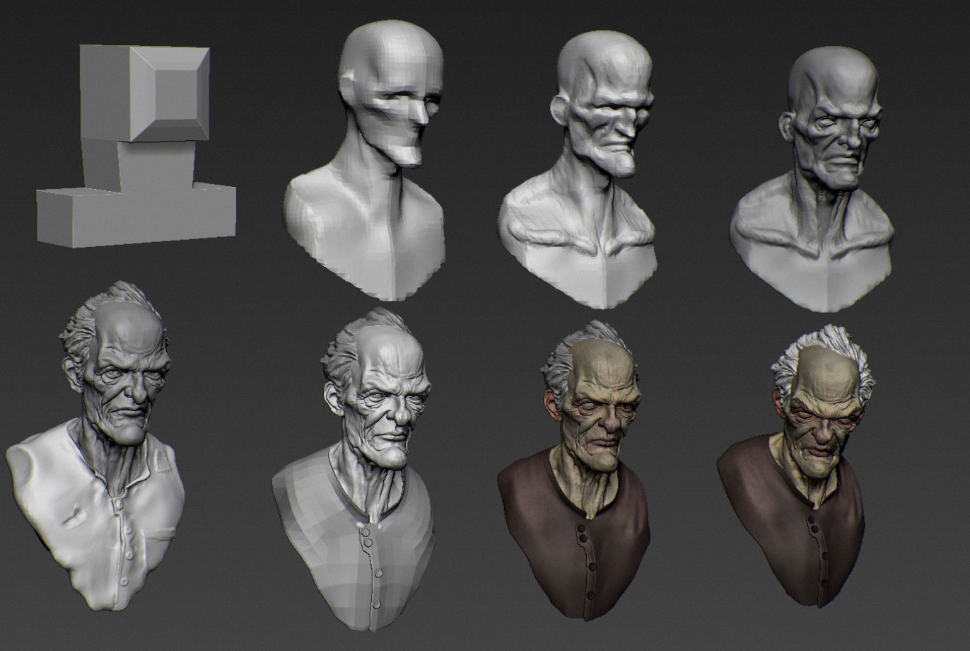
During the whole process, quad meshes are often preferable by artists because they often provide good edge flows that better represent curvatures and features of shapes. In comparison to a triangle mesh, the subdivided quad mesh often have better topologies with lesser irregular vertices and it’s also easier for deformation and texture export algorithms to work with quad meshes. That’s why a varieties of approaches developed to help artists build quad or quad dominant meshes from scratch to serve as a good base mesh for further steps in the modelling pipeline.

Traditionally, artists often use curves/surfaces like Bezier, B-Spline or Nurb to create patches aligned to each other to form the coarsest base meshes. The approach is quite unintuitive because it requires artists to adjust control points to change the surface and it’s also quite hard to match multiples surface patches together. Another approach makes use of polygon operators like extrude, inset, bevel, etc. to add quads to base mesh step by step. However, this is a time-consuming task, and because artists are busy with manipulating individual quads, it is hard for them to focus on the overall shape. That’s why skeleton-based modeling comes into the scene as a good method for building rough base meshes.

Skeleton, like ones of human and animals, due to its nature, could help represent the principal shape of 3D objects better. In the context of modeling, a skeleton is the union of cone-spheres like depicted in Figure 2. Cone-spheres, as defined (Barbier, et al., 2004), is a cone limited by two spheres at its both ends. Artists could adjust the radius of two spheres to inflate and deflate the cone-sphere or move the position of spheres to change the pose of a skeleton. Because they do not have to manipulate individual vertices and quads of the base mesh, the modeling process is faster and more intuitive.

Technically, a skeleton is a graph consisting of nodes and edges. Each node is a sphere defined by a point and a radius, connected to other ones by edges. Nodes with more than 2 adjacent edges are called branch nodes, nodes with two adjacent nodes are called connection nodes, nodes with only one adjacent node called end nodes, and nodes with no adjacent node at all are called isolated nodes. We also call an edge connecting two branch nodes are branch edges and edges along paths from branch to end nodes are end edges. Algorithms will use the geometric and topological information to construct the approximated meshes.

In this article, we will first summarize the previous works on skeleton-based modeling and then, explain in detail our implementation in Blender and finally, summarize the result and explain limits that we haven’t been able to solve yet.

Previous work

Generally, algorithms that convert skeletons into quad-dominant meshes often do three things: build a polyhedron for the sphere of each branch node and also tubes around skeleton edges, stitch the tubes to polyhedrons, and evolve the vertices of the mesh toward the surface of conespheres.

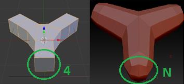
Intuitively, the current algorithms could be classified into two main types characterized by the number of quads at each cross-section of tubes around skeleton edges. As described in Figure 3, the first one tries to impose four quads around edges, so stitching between tubes and polyhedrons of branch nodes become trivial. The second type allows the number of quads to be variable, which causes a need to balance the amount so the tubes can be stitched to the polyhedron.

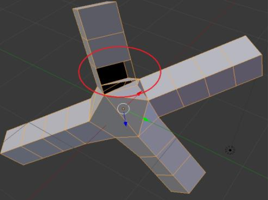
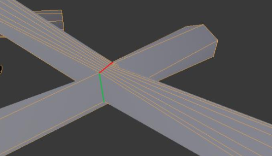
The method proposed by (Ji, et al., 2010) belongs to the first type of algorithm. It was integrated into Blender years ago and is still widely used by Blender artists. It starts by marching a quadrangular frame along skeleton edges, creating one quadrangular tube around each edge. Next, it collects a set of the quadrangular frames around each branch node, one frame for each adjacent edge. The frames will be used to construct a convex hull around the branch node. For the edge tubes to be stitched to the convex hull, triangles on the convex hull need to be collapsed into quads, so there could be one quadrangular slot for each edge tube. Unfortunately, as collapse depends on the number of triangles and their geometry, it is not always correct that all triangles could be merged into quads; therefore, some tubes could be left with no slot. As in Figure 4, the method failed even at a branch node of 4 adjacent edges. However, artists still prefer the method because the resulting meshes of quadrangular tubes are very coarse. Moreover, in combination with a subsequent subdivision step, the tubes result in very organic models. Thanks to the quadrangular tubes, artists could create other hard models like guns, chairs, etc. rather than just organic models.

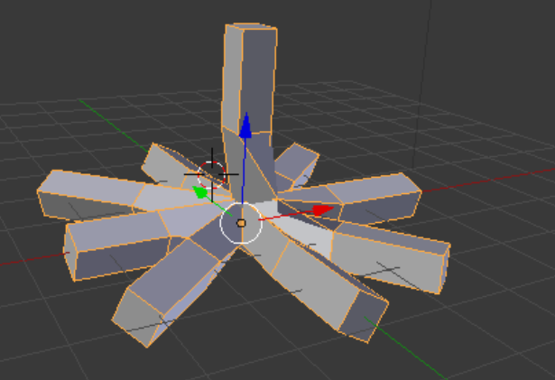
Also belonging to the first type of algorithm, a recent method (Panotopoulou, et al., 2017) solved the stitching problem mentioned above. Given a set of intersection points between adjacent edges and the sphere of each branch node, it first cuts the sphere into spherical quads, one for each adjacent edge. To be more specific, from the first three points, there are always two antipodal points that are equidistant the three points. Connecting the two antipodal points with three geodesic curves through the center of the arc between each pair of intersection points, we will have the first three spherical quads, one for each edge. For each next intersection point, for example, the 4th point, the method finds a created spherical quad containing the 4th point, insert a new point at the center of the arc between the 4th point and the point of the spherical quad, and split the quad into two more smaller ones by connecting the new point to one of its diagonals. By repeating the process until there is no intersection point left, the method ensures that each adjacent edge has its own spherical quad, and therefore, is always stitched to the branch node. Unfortunately, the method suffers from another problem that the positions of spherical quads are often distorted and in some cases, the four-quad topology is not enough to represent the shape as depicted in Figure 5.

Classified as the second type of algorithm, the method (Fuentes Su{'a}rez, et al., 2017) starts by building a Voronoi diagram for the sphere of each branch node. The Voronoi diagram consists of multiple cells, one for each adjacent edge of the branch node. The number of vertices of each Voronoi cell, which we call the degree of Voronoi, varies depending on the number of adjacent Voronoi cells. When two branch nodes are connected to each other by a skeleton edge, for them to be stitched, the degrees of two Voronoi cells at both ends of the end have to be identical. Therefore, when the degrees are unequal, the method has to balance them by inserting points at Voronoi edges of the Voronoi cells of lower degree. However, the method doesn’t suggest a way to optimize the number of insertion, it just instead split random edges of Voronoi cells until their degrees are equal, which makes the final mesh sometimes very dense. Another problem is that the method doesn’t prove that if the approach could terminate when cycles exist in skeletons.

A recent research suggests a way to solve these two above problems by integer linear programming. As we know, increasing the degree of one Voronoi cell is done by splitting its edges, for example, if we need to increase the degree from 6 to 9, we can choose split one of its edges one time and two times at another edge. The method calls the number of splitting the weight of a Voronoi edge. Therefore, the problem will come down to optimize the total integer weight of all Voronoi edges on branch nodes of the skeleton with the constraint that the total edge weight of cells at both ends of branch edges are equal. Unfortunately, although the approach helps reduce the number of splitting, it results in an uneven distribution of subdivision at edges of Voronoi cells, as seen in Figure 6. For instance, some edges could be split many times while some other ones are untouched at all. Consequently, the n-quads tubes around skeleton edges could be very dense on some sides and sparse in other sides. One reason behind it is that some Voronoi edges are preferable for splitting because they are shared between two Voronoi cells of lower degree.

Therefore, splitting them will increase the degrees of both Voronoi cells. It is like “Kill two birds with one stone”. Another reason is that some Voronoi edges shared by Voronoi cells belonging to a skeleton end edges (edges connected to end nodes). Splitting these edges will just ONLY increase the degree of the Voronoi cells. In other words, it won’t increase the degree of Voronoi cells of branch edges, whose degrees are already higher than ones at the other end

Selected Approach

Each method summarized above has its own strengths and weaknesses. The method B-Skin (Ji, et al., 2010) is integrated into Blender years ago and even the implementation suffers from the problem of stitching quadrangular tubes to the convex hull of branch nodes, artists are still able to work around it by carefully adjusting positions of branch nodes and their adjacent nodes. Although the method (Panotopoulou, et al., 2017) helps solve the stitching problem, it creates a more severe problem relating to positions of quadrangular slots on branch nodes, as depicted in Figure 5. Therefore, it’s unlikely that Blender artists will prefer this new one.

While waiting for further research on the problem, it would be more beneficial to provide Blender artists with a different style of mesh by applying the second type of algorithm. It will coexist with the current implementation, so the artists could go back and forth between different algorithms to find out which is the better ones.

Between two methods that produce n-quads tubes around skeleton edges, I prefer to use the one (Bærentzen, et al., 2012) because even it could not process cyclic skeletons and the resolution is a bit dense, the quad distribution at each cross-section around skeleton edges are more even, which is preferable by artists. The remaining part of the article will be used to describe in detail the implementation.

Implementation

The input to the implementation is a graph, as mentioned above, defined by nodes and edges. Each node owns an adjacent edge list and the geometry information including a sphere radius and position. The output will be a quad-dominant mesh, which should contain as many quads as possible. The mesh is defined by the B-Mesh data structure of Blender. The implementation runs through four main steps.

• From the input skeleton, build a graph called SQM. Nodes of SQM graph are only branch nodes, end nodes, and isolated nodes from the input skeleton graph. Each SQM edge contains a list of connection nodes between branch nodes or end nodes. The list could be empty when there are no connection nodes between them.
• Build a Voronoi diagram for the sphere of each branch node.
• Balance the degrees of Voronoi cells.
• Stitch branch nodes and end nodes.
• Evolve the mesh to the original surface of cone-spheres.

Build SQM graph

Why do we need to build another graph from the input skeleton? The answer is that the SQM algorithm requires us to process queries like what is another branch node linked to this branch node, or what are connection nodes lying between these two end nodes, etc. To answer these queries, from one branch node, we have to perform a deep first search until we encounter another adjacent branch node, which could take more time and make the code hard to understand. Therefore, building another graph that stores only branch and end nodes would be more beneficial. In Figure 7, the left graph is the input skeleton and the right one is the SQM graph.

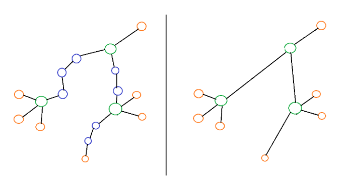
To build an SQM graph, we perform a deep first search on the skeleton. When first coming across an end node or branch node, we created a new SQM node and a list of new SQM edges corresponding to the number of adjacent edges of the node. Along the search, if the next node is a connection node, we add the node to the connection node list of the SQM edge. Otherwise, if the next node is an end or branch node, we finish an SQM edge.

Build a Voronoi diagram for the sphere of each branch node

To build a Voronoi diagram, we first need to build a convex hull from a set of intersection points between the sphere of a branch node and its adjacent edges. When all points are planar, we need to joggle some point a bit to make them un-planar, so the dimension of the point set will be three. We call vertices of the convex hull are path vertices, each of which corresponds to an end or branch edge. Path vertices will be assigned to SQM edges they belong to; therefore, an SQM edge between two branch nodes will have two path vertices on two convex hulls; while an SQM edge between a branch node and an end node will have only path vertex.

To create a Voronoi cell for each path vertex, we split each of its adjacent triangles into six smaller triangles as illustrated in Figure 8. After splitting, each path vertex will be isolated from other ones; therefore, we can delete it and all of its adjacent triangles to make a hole slot, serving as a placeholder for stitching.

Balance the degrees of Voronoi cells

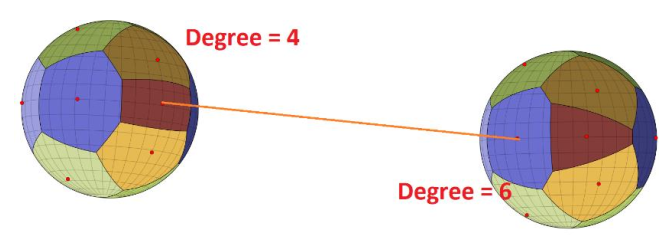
To stitch branch nodes at both ends of an SQM edge, the degrees of the two Voronoi cells of two path vertices have to be equal, which means existing a one-one mapping between vertices; otherwise, we will end up creating triangles. We find the SQM edges whose Voronoi degrees at both ends are unequal, as depicted in Figure 9, to balence. Increasing the degree of Voronoi cell means increasing the valence of its path vertex, which is done by splitting its opposite edges in its adjacent triangles, as seen in Figure 8. For a better uniform distribution of vertices around path vertices, we select the longest opposite edge to split at each iteration.

Stitch branch nodes and end nodes

After all Voronoi cells at ends of SQM branch edges have equal degrees, we can process them one by one. For each SQM edge, we start from one path vertex, collect the ring of vertices around it and then march the ring along skeleton nodes of the SQM edge. If the other node of the SQM edge is another branch node, we stitch the marching ring to the ring of vertices around the other path vertex; otherwise, if it is an end node, we close the ring by connecting its vertices to one central point. The result will be a tube around the edge with the number of quads at a crosssection is equal to the number of vertices of the marching ring, as in Figure 10.

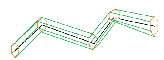
There are two main problems we need to solve in the process. First, generating a ring of vertices around each connection node on the SQM edge. Second, given two rings of vertices, find an order to stitch them together.

The ring of vertices at each connection node could be generated along an eclipse, which is the intersection between two cone-spheres at the node. The eclipse is defined by two axes, one is the bisector vector of two edges and the other is the vector perpendicular to the plane of two edges.

For stitching two rings to each other, we need to match vertices on two rings into pairs so that the segment of each pair is parallel to the axis between two nodes as much as possible. To achieve that, we keep a ring still and rotate the other ring, actually, it’s just a rotation shifting of indices. We will choose the rotation of the smallest total distance between two rings.

Move the positions of vertices to the original surface

Until now, we have a mesh that could represent quite well the shape of skeletons made by conespheres. Now, we need to project the mesh’s vertices onto the surface of cone-spheres. This is not a trivial task because when cone-spheres are overlapped too much, their intersections are very far from the spheres of branch nodes, where the original vertices we need to move stay on. The following implementation just uses an approximated method to do it.

For vertices on the body of cone-spheres that are already quite near to the expected surface, we just need to find the nearest point to the surface from each vertex. Now, we only consider the cases when vertices on branch nodes with a number of adjacent vertices, some of which could be on the same branch node; while some other could be on other nodes. We call adjacent vertices on other nodes are on-node adjacent vertices. Based on this observation, we could classify these vertices depending on the number of vertices on other nodes and devise specific ways to handle each type of vertex, as depicted in Figure 11

• For vertices with three on-node adjacent vertices, the best position is the intersection point between two cone-spheres. Unfortunately, we haven’t found out a way to find that point and ends up approximating it by averaging the intersection between three pairs of cone-spheres.
• Vertices with two on-node adjacent vertices, it’s possible that they lie on the ellipse intersection between two cone-spheres.
• Vertices with one on-node adjacent vertex, it’s likely that they lie on the body of one conesphere, so we could project them on the cone-sphere.
• Vertices with no on-node adjacent vertex could be assumed that they do not lie on intersection regions between cone-spheres, and we could safely project them onto the sphere of the branch node

Conclusion and further works

The implementation of the SQM method is integrated into Blender but still in the process of review for publishing to the main repository. Technically, the implementation could process skeleton of hundreds of nodes in real time, not slower than the current implementation of the method B-Skin (Ji, và những tác giả khác, 2010) in Blender. It is also able to handle a variety of cases when the shape of skeleton changes hugely. From the user aspect, some artists volunteered in creating a variety of organic models using the feature. Although it couldn’t produce better organic models than the current method, it solved the problem of stitching branch nodes, which quite frustrates the Blender artists. With the method, the artists could model objects with multiple branches like human hands, starfishes, etc. more effectively than the current method. Therefore, it could be used in parallel with the current implementation, as an alternate option.

One problem of current implementation is at projecting the vertices on the surface of conespheres. The current approach presented above is quite unstable when adjacent cone-spheres are overlapping too much. The vertices on the spheres are very far from the real surface and we haven’t found a good direction to move these vertices to the real surface. Moreover, branch vertices with three on-node adjacent vertices haven’t been handled correctly, which makes the result unpredictable when three cone-spheres overlap too much. In the future, in addition to finding a better way to projecting vertices precisely onto the actual surface of cone-spheres, we also want to change our approach to just moving vertices approximately, so the result could be acceptable to artists. This is because artists, in fact, don’t see the cone-spheres directly, they instead just adjust the radius until they feel satisfied. Therefore, projecting vertices onto surface of cone-spheres will be unnecessary.

We also want to study more about how to optimize the number of splitting at edges of Voronoi regions with the constraint that the number of insertion points is distributed evenly on edges.

References

• Bærentzen J. A., Misztal M. K. and Wełnicka K. Converting skeletal structures to quad dominant meshes

• Barbier Aurelien and Galin Eric Fast Distance Computation Between a Point and Cylinders, Cones, LineSwept Spheres and Cone-Spheres

• Fuentes Su{'a}rez Alvaro Javier and Hubert Evelyne Scaffolding skeletons using spherical Voronoi diagrams

• Ji Zhongping, Liu Ligang and Wang Yigang B-Mesh: A Modeling System for Base Meshes of 3D Articulated Shapes

• Panotopoulou Athina [et al.] Scaffolding a Skeleton

Contact

if you have further question about the features, you can contact me through my email khanhhh89@gmail.com