Image-Based Virtual Try On Network - Part 1
- Overview
- Geometric Matching Module
- How is the Thin Plate Spline (TPS) transformation generated?
- Conclusion
Overview
In this article, I explain in detail the idea behind the paper “Toward Characteristic-Preserving Image-based Virtual Try-On Network” in the field of image-based virtual try-on that puts clothes on human subjects. The main stages of the pipeline are described in parallel with the Pytorch implementation provided by the author.
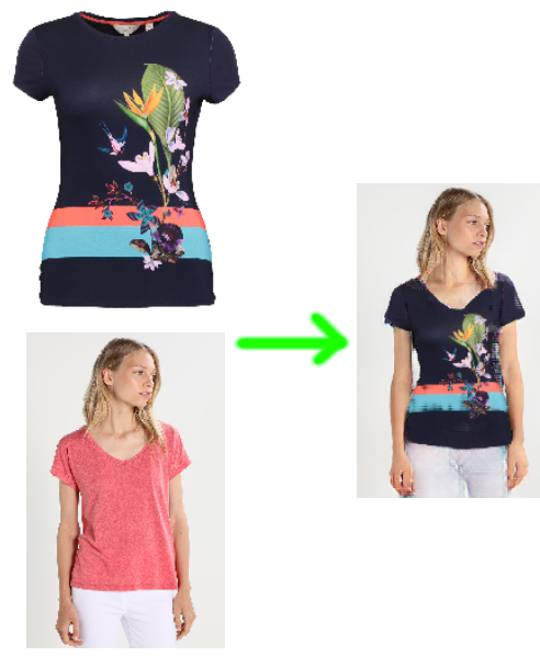
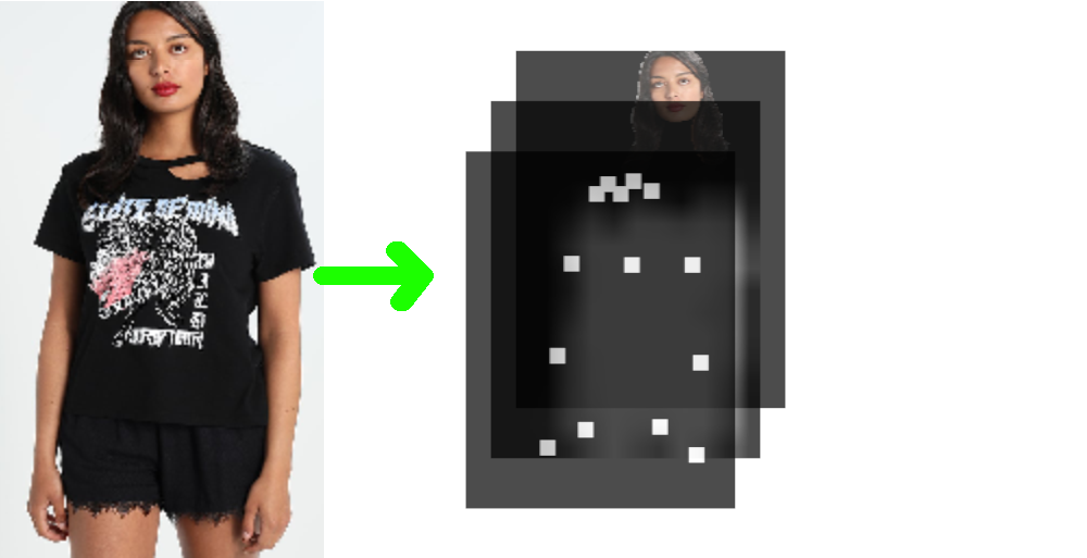
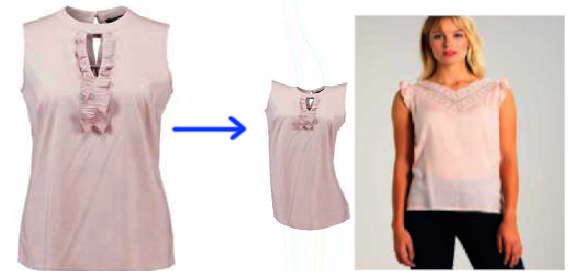
The below picture illustrates the general idea of the image-based virtual try on problem. Given two input images: the in-shop cloth and a person in similar pose, the problem is putting the in-shop cloth on the human subject, as shown in the right side of the picture.
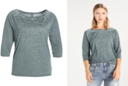
The training data used in this paper consists of the image of a human target wearing a cloth and the corresponding in-shop picture of that cloth. These pairs of images could be found abundantly in the websites of clothes shops. One example pair is shown in below.
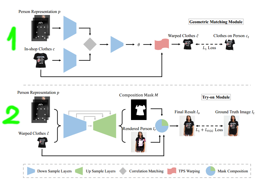
According to the paper, the general pipeline consists of two main stages.
The first stage trains a module called Geometric Matching Module to predict a thin plate spline deformation that warps the in-shop cloth image to match the corresponding cloth on the model image. After training is done, the model is used to deform/warp all the input in-shop clothes images, which will be used as the training data for the next stage.
The second stage trains another module called Try-On to put the warped clothes on the human subject. Instead of predicting directly the final result, this module predicts a rendered person image and a composition mask separately and then use the mask to blend the rendered person image with the input warped image to form the final result.
Due the length of the pipeline, I will first focus on explaining the first stage in this article and save the second stage for the next article.
Geometric Matching Module
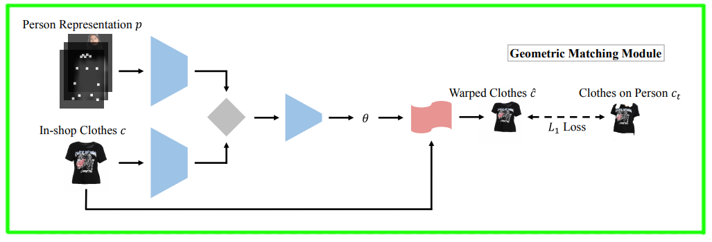
From two input data: standard in-shop clothes image $c$ and a person representation $p$ , the module GMM learns to warp the clothes image so that it aligns with the target pose in the person image.
Calculate person representation: $p$
The person image is not passed to the model directly because in the test time this image is not available. Therefore, the input person is image is transformed to another person representation to get rid of information about old clothes, color, texture and shape and still preserves face, hair and general body shape of the target. As described in the section 3.1 in the paper, the human representation consists of
- A pose heat map is a 18-channel image where each slice encodes the heat map of a skeleton joint.
- A body shape map is 1-channel image which describes the blurred shape of the person.
- An RGB image that contains the facial and hair region of the human subject.
Find feature correlation
After the person representation $p$ is extracted from the input image, with the cloth image $c$, they are passed to two separate feature extraction modules, each of which consists of a chain of 2-strided down-sampling convolutional, batch normalization and relu layers, as shown in below.
class FeatureExtraction(nn.Module):
    def __init__(self, input_nc, ngf=64, n_layers=3, norm_layer=nn.BatchNorm2d, use_dropout=False):
        super(FeatureExtraction, self).__init__()
        downconv = nn.Conv2d(input_nc, ngf, kernel_size=4, stride=2, padding=1)
        model = [downconv, nn.ReLU(True), norm_layer(ngf)]
        for i in range(n_layers):
            in_ngf = 2**i * ngf if 2**i * ngf < 512 else 512
            out_ngf = 2**(i+1) * ngf if 2**i * ngf < 512 else 512
            downconv = nn.Conv2d(in_ngf, out_ngf, kernel_size=4, stride=2, padding=1)
            model += [downconv, nn.ReLU(True)]
            model += [norm_layer(out_ngf)]
        model += [nn.Conv2d(512, 512, kernel_size=3, stride=1, padding=1), nn.ReLU(True)]
        model += [norm_layer(512)]
        model += [nn.Conv2d(512, 512, kernel_size=3, stride=1, padding=1), nn.ReLU(True)]

        self.model = nn.Sequential(*model)
        init_weights(self.model, init_type='normal')

    def forward(self, x):
        return self.model(x)
Both extracted features are then passed to a correlation module that is supposed to merge them into a single tensor that encodes the correlation between the person pose and the standard in-shop clothes. Specifically, assume that $1$ is the feature map from the person representation $p$, and $2$ is the feature map from the in-shop cloth $c$, each feature column in the feature map $3$ encodes the similarities between the corresponding feature column in $2$ and every other feature columns in $1$. In other words, the correlation map $3$ encodes the pairwise similarity between two feature maps $1$ and $2$. Please check this lecture for further explanation about this mechanism.
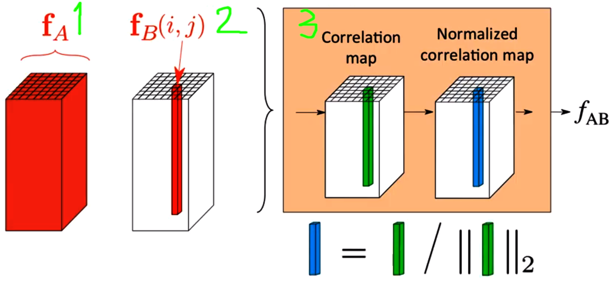
The code for calculating the correlation map $3$ is shown in below.
class FeatureCorrelation(nn.Module):
    def __init__(self):
        super(FeatureCorrelation, self).__init__()

    def forward(self, feature_A, feature_B):
        b,c,h,w = feature_A.size()
        # reshape features for matrix multiplication
        feature_A = feature_A.transpose(2,3).contiguous().view(b,c,h*w)
        feature_B = feature_B.view(b,c,h*w).transpose(1,2)
        # perform matrix mult.
        feature_mul = torch.bmm(feature_B,feature_A)
        correlation_tensor = feature_mul.view(b,h,w,h*w).transpose(2,3).transpose(1,2)
        return correlation_tensor
Predict Thin-Plate-Spline transformation
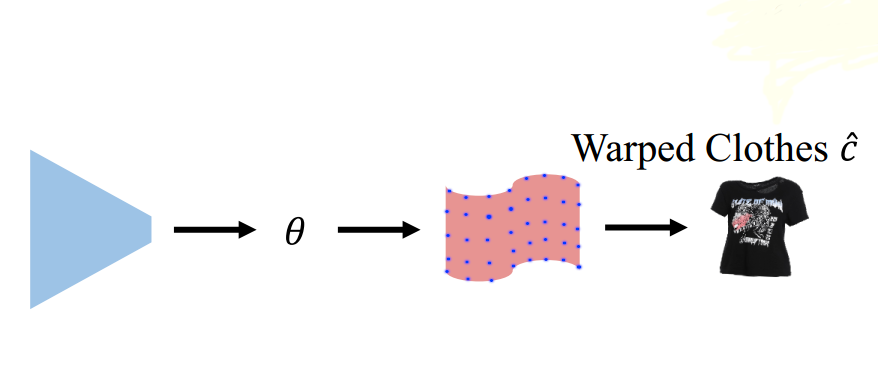
The correlation map is then passed to a regressor (the blue trapeze block) that predicts the warped control points for the Thin-Plate-Spline stage, as depicted by the blue points in the below figure. These blue control points will be then used to solve for a smooth Thin-Plate-Spline transformation that warps the input in-shop clothes images to align with the target clothes images on the human subject. In other words, the Thin-Plate-Spline transformation is learned by minimizing the MSE loss between the warped clothes and the corresponding target clothes.
The complete code from feature extracting to grid prediction is shown in below.
# construct the regressor
self.regression = FeatureRegression(input_nc=192, output_dim=2*opt.grid_size**2, use_cuda=True)

# extract features from person representation and in-shop clothes image
featureA = self.extractionA(inputA)
featureB = self.extractionB(inputB)
featureA = self.l2norm(featureA)
featureB = self.l2norm(featureB)
# combine two features A and B into a correlation tensor
correlation = self.correlation(featureA, featureB)
# pass the correlation tensor to the regressor to predict warped control points for the Thin-Plate-Spline stage
theta = self.regression(correlation)
grid = self.gridGen(theta)
How is the Thin Plate Spline (TPS) transformation generated?
General idea
In this part, I will go deeper into explaining how the TPS transformation is generated because it seems that it is the most important step in the Geometric Matching Module.
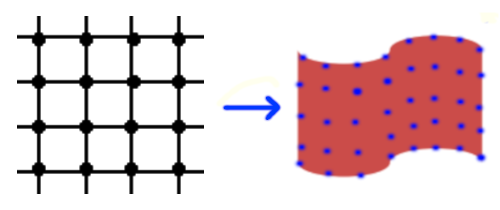
Given two sets of grid control points, the module TpsGridGen estimates a Thin Plate Spline transformation that warps the in-shop clothes to match the person pose.
The first control point set, as shown in the left picture, is constructed in the initialization stage and does not change during the training process. The second control point set in the right picture is the prediction result from the regressor, as represented by the tensor variable theta in the previous code.
Actually, the two set of control points will serve as the input and the target set to estimate parameters $a_1, a_x, a_y, w_i$ of the thin plate transformations. For further explanation about these two equations, please check my previous article about TPS.
The estimated TPS transformation will be then used to sample a dense pixel mapping, which maps the pixels in the in-shop clothes image to the pixels in the domain of the target clothes image so that the final warped clothes image aligns with the human subject.
Implementation
The main stages of the TPS transformation estimations are explained in below.
In the initialization stage, the first control point set are constructed as follows. The tensor T_x and T_y stores the $x$, $y$ coordinates of grid points.
#grid_size: the number of control points along each dimension.
axis_coords = np.linspace(-1,1,grid_size)
#N: the total number of control points
self.N = grid_size*grid_size
P_Y,P_X = np.meshgrid(axis_coords,axis_coords)
P_X = np.reshape(P_X,(-1,1)) # size (N,1)
P_Y = np.reshape(P_Y,(-1,1)) # size (N,1)
P_X = torch.FloatTensor(P_X)
P_Y = torch.FloatTensor(P_Y)
This control point set is used to construct the matrix $L$ that defines the left hand side of the linear system to solve for coefficients of the TSP transformations. Here we just glimpse quickly over the matrix L.
As an example, the matrix L for a set of 3 control points will looks like as follows.
The sub-matrix $K$ defines the pairwise distance between each control point and the TPS kernels of every other control points. For the example, its first row $\begin{bmatrix}K_{00} & K_{10} & K_{20}\end{bmatrix}$ specifies the distances between the points $P_0, P_1, P_2$ to the TPS kernel of the control point $P_0$. Each $K_{ij}$ is calculated based on the following equation.
where U is the kernel function $U(r) = r^2log(r)$.
The column vector $[w \ \ a]^T$ denotes the coefficients of the TPS transformation. Because we solve for two transformation functions, one for $x$ mapping and one for $y$ mapping, our final TSP transformations will be two column vectors $ W_x = [w \ \ a]^T$ and $W_y = [w \ \ a]^T$
The sub-matrix $P$ is formed by stacking control points vertically and the sub-matrix $O$ is zero matrix.
The right hand side of the system $Y’ = [y_0’\ y_1’\ y_2’\ 0\ 0\ 0]^T$, or $X’ = [x_0’\ x_1’\ x_2’\ 0\ 0\ 0]^T$ denotes the target control point coordinates $y_i$ and $x_i$, which are predicted by the regression module, as explained the previous section. When these two vectors $X’$ and $Y’$ are available to us in the training time, the coefficient vector $W_x$ of the $f_x’$ interpolator and the coefficient vector $W_y$ of the $f_y’$ interpolator could be calculated as
With these equations in mind, the construction of the matrix L is shown below.
#X: Nx1 array that represents the x coordinates of the control point set.
#Y: Nx1 array that represents the y coordinates of the control  point set.
def compute_L_inverse(self,X,Y):
    N = X.size()[0] # num of points (along dim 0)
    # construct matrix K
    Xmat = X.expand(N,N)
    Ymat = Y.expand(N,N)
    # a quick way to calculate distances between every control point pairs
    P_dist_squared = torch.pow(Xmat-Xmat.transpose(0,1),2)+torch.pow(Ymat-Ymat.transpose(0,1),2)
    P_dist_squared[P_dist_squared==0]=1 # make diagonal 1 to avoid NaN in log computation
    #the TPS kernel function $U(r) = r^2log(r)$
    K = torch.mul(P_dist_squared,torch.log(P_dist_squared))
    # construct matrix L
    O = torch.FloatTensor(N,1).fill_(1)
    Z = torch.FloatTensor(3,3).fill_(0)
    P = torch.cat((O,X,Y),1)
    L = torch.cat((torch.cat((K,P),1),torch.cat((P.transpose(0,1),Z),1)),0)
    Li = torch.inverse(L)
    if self.use_cuda:
        Li = Li.cuda()
    return Li
The inverse matrix $Li$ will be saved for calculating TPS coefficients in the forward step.
self.Li = self.compute_L_inverse(P_X,P_Y).unsqueeze(0)
In the training time, given the output $\theta$, the control point displacements, predicted by the regressor, the coeffient vector $W_x, W_y$ are calculated as follows.
# extract the displacements Q_x and Q_y from theta
Q_X=theta[:,:self.N,:,:].squeeze(3)
Q_Y=theta[:,self.N:,:,:].squeeze(3)
# add the displacements to the original control points to get the target control points
Q_X = Q_X + self.P_X_base.expand_as(Q_X)
Q_Y = Q_Y + self.P_Y_base.expand_as(Q_Y)

# multiply by the inverse matrix Li to get the coefficient vector W_X and W_Y
W_X = torch.bmm(self.Li[:,:self.N,:self.N].expand((batch_size,self.N,self.N)),Q_X)
W_Y = torch.bmm(self.Li[:,:self.N,:self.N].expand((batch_size,self.N,self.N)),Q_Y)
The coefficient vector $W_x, W_y$ are estimated from two sparse control point set, but what we need to warp the input in-shop clothes is a dense pixel mapping. This is achieved by plugging all pixel indices $(x,y)$ in the input domain to the two interpolators $f_x’, f_y’$ .
The code to achieve it is shown in below. I cut off some reshape operations from the code for the sake of clearance.
#calculate the linear part a_1 + a_x*a + a_y*y
A_X = torch.bmm(self.Li[:,self.N:,:self.N].expand((batch_size,3,self.N)),Q_X)
A_Y = torch.bmm(self.Li[:,self.N:,:self.N].expand((batch_size,3,self.N)),Q_Y)

# here points are our dense grid point set.
# compute distance P_i - (grid_X,grid_Y)
# grid is expanded in point dim 4, but not in batch dim 0, as points P_X,P_Y are fixed for all batch
points_X_for_summation = points[:,:,:,0].unsqueeze(3).unsqueeze(4).expand(points[:,:,:,0].size()+(1,self.N))
points_Y_for_summation = points[:,:,:,1].unsqueeze(3).unsqueeze(4).expand(points[:,:,:,1].size()+(1,self.N))

# pass the distances to the radial basis function U
dist_squared = torch.pow(delta_X,2)+torch.pow(delta_Y,2)
# U: size [1,H,W,1,N]
dist_squared[dist_squared==0]=1 # avoid NaN in log computation
U = torch.mul(dist_squared,torch.log(dist_squared))

# finally
# multiply the kernel distances U with the nonlinear coefficients
# add it with the liear part
points_X_prime = A_X[:,:,:,:,0]+ \
               torch.mul(A_X[:,:,:,:,1],points_X_batch) + \
               torch.mul(A_X[:,:,:,:,2],points_Y_batch) + \
               torch.sum(torch.mul(W_X,U.expand_as(W_X)),4)

points_Y_prime = A_Y[:,:,:,:,0]+ \
               torch.mul(A_Y[:,:,:,:,1],points_X_batch) + \
               torch.mul(A_Y[:,:,:,:,2],points_Y_batch) + \
               torch.sum(torch.mul(W_Y,U.expand_as(W_Y)),4)

# concatenate dense array points points_X_prime and points_Y_prime
# into a grid
return torch.cat((points_X_prime,points_Y_prime),3)
With the warped dense grid points, we can use the pytorch function F.grid_sample to warp the input in-shop clothes, input grid points for the sake of debugging as below.
#grid the result returned from the previous code.
grid, theta = model(agnostic, c)
# c is the in-shop clothes image
warped_cloth = F.grid_sample(c, grid, padding_mode='border')
# img_g is a image with drawn grid points
warped_grid = F.grid_sample(im_g, grid, padding_mode='zeros')
Conclusion
In this article, I explained about the Geometric Matching Module in the paper that predicts a Thin Plate Spline Transformations used to warp the input in-shop clothes image to match the pose of a target person. For explanation about the second stage of the paper, the virtual module, that actually put the warped clothes on the human subject, please check my next article.