Learning 3D Human Dynamics From Video
- Introduction
- Overview
- Learn 3D dynamics representation $\Phi_t$
- Learn 3D human mesh representation $f_{3D}$
- Learn Delta Pose Regressor $f_{-\Delta{t}}$ and $f_{\Delta{t}}$
- Generator-Discriminator mechanism.
- Dynamics learning losses
- Conclusion
Introduction
In one of last articles, I summerized the paper “End-to-end Recovery of Human Shape and Pose” which predicts the 3D shape and pose of a human subject from a single image in a weak-supervised manner. This paper “Learning 3D Human Dynamics from Video” pushes the human estimation problem further by learning the 3D dynamics of a human subject from an input video, which, as stated by the author, helps increase the stability of the 3D prediction result.
All the code and pictures presented in this article is taken from the author’s paper and code repository.
Overview
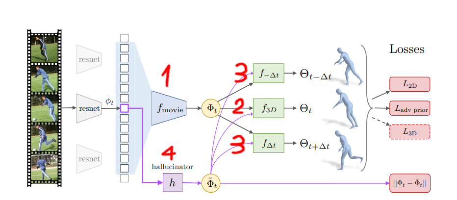
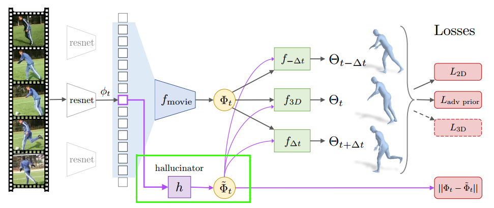
From my understanding, there are four main types of models that forms the backbone of the architecture, as annotated in the above figure.
First, a temporal encoder $f_{movie}$ is trained to learn the temporal 3D dynamics representation (movie strip) $\Phi_t$ from a temporal sequence of images.
Second, the temporal 3D dynamics representation or movie strip $\Phi_t$ is used to train $f_{3D}$, a regressor that predicts shape, pose and camera parameters of the human subject at the center frame.
Third, to enforce that the movie strip $\Phi_t$ truly encodes the 3D dynamics of the subject, delta regressors $f_{t+\Delta{t}}$ are trained to predict the change in pose from the frame $t$ to $t-\Delta{t}$ or $t+\Delta{t}$. From my understanding, these regressors serve as cross-checking mechanism that force temporal relations, from pose $\theta_{t-\Delta{t}}$ to pose $\theta_{t}$ or vice versa, are integrated into $\Phi_t$.
Finally, the paper suggests a regressor called $Hallucinator$ that predicts $\Phi_t$ from a single image feature $\phi_t$. According to the author, this regressor could be used to predict the past and future movements of a human subject from a single image.
Learn 3D dynamics representation $\Phi_t$
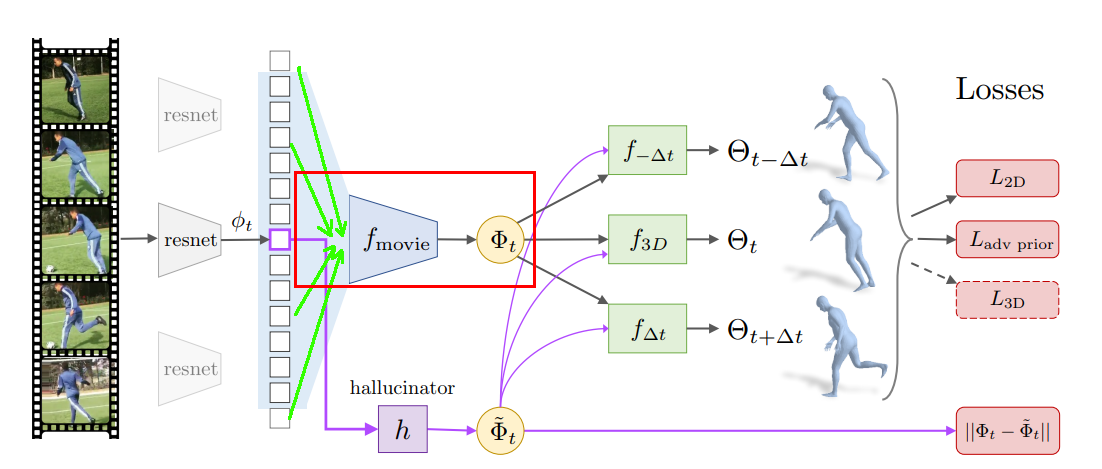
The temporal encoder, which is highlighted by the red rectangle in the above figure, is a series of 1D convolutional layers that learn a representation $\Phi_t$ (Phi) denoting the 3D dynamics of the human subject from a sequence of temporal image features. The input to this module is a concatenation of image features $\phi_t$, each of which is extracted from encoders like Resnet, etc.
As shown in the below code, the Resnet encoder $f_image_enc$, which is pretrained on a single 3D human pose and shape prediction task, transforms a temporal sequence of input images $I_t$ to image features called $img_feat_full$ of size $B\times T\times F$ where $B$ is the batch size, $T$ is the sequence length, and $F$ is the feature length from Resnet. To reduce the training time, the code also supports loading pre-extracted features from $self.phi_loader$
print('Building model..')
if not self.precomputed_phi:
    print('Getting all image features...')
    # Load all images at once. I_t should be B x T x H x W x C
    I_t = self.image_loader[:, :]
    # Need to reshape I_t because the input to self.f_image_enc needs
    # to be B*T x H x W x C.
    I_t = tf.reshape(I_t, (self.batch_size * self.sequence_length,
                           self.img_size, self.img_size, 3))
    img_feat, phi_var_scope = self.f_image_enc(
        I_t, weight_decay=self.e_wd, reuse=tf.AUTO_REUSE)
    self.img_feat_full = tf.reshape(
        img_feat, (self.batch_size, self.sequence_length, -1))
else:
    print('loading pre-computed phi!')
    # image_loader is B x T x 2048 already
    self.img_feat_full = self.phi_loader
The learned image features $self.img_feat_full$ or $(\phi_{t-\Delta{t}}, … \phi_{t}, … ,\phi_{t+\Delta{t}})$ are passed to the temporal encoder $self.f_temporal_enc$ to learn the dynamics of the human subject $\Phi_t$ as in below.
movie_strip = self.f_temporal_enc(
    is_training=True,
    net=self.img_feat_full,
    num_conv_layers=self.num_conv_layers,
)
The function $self.f_temporal_enc$ applies $num_conv_layers$ of convolutional layers to the temporal image features and produces the representation of 3D dynamics $\Phi_t$ whose size is $T\times 2018$. The architecture is shown in the below code.
#az_fc2_groupnorm is self.f_temporal_enc in the above code snippet.
def az_fc2_groupnorm(is_training, net, num_conv_layers):
    """
    Each block has 2 convs.
    So:
    norm --> relu --> conv --> norm --> relu --> conv --> add.
    Uses full convolution.


    Args:
    """
    for i in range(num_conv_layers):
        net = az_fc_block2(
            net_input=net,
            num_filter=2048,
            kernel_width=3,
            is_training=is_training,
            use_groupnorm=True,
            name='block_{}'.format(i),
        )
    return net
Learn 3D human mesh representation $f_{3D}$
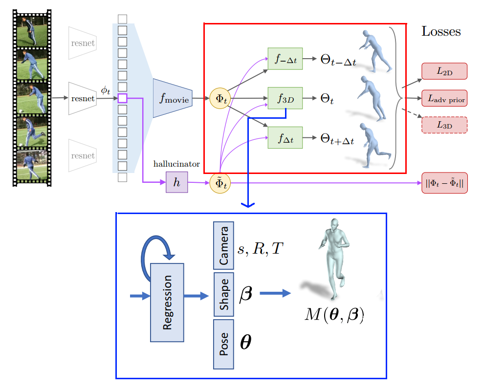
The 3D dynamics representation $\Phi_{t}$ $T \times 2048$ described in the below paragraph just contains a general, raw data about the shape, camera and pose changes within the temporal window. This information cannot be used to pass in the SMPL model to reconstruct the 3D mesh format of the human subject. To do it, another regressor $f_{3D}$ is trained to predict the 3D mesh representation of the human subject $\Theta_t$, which is depicted in detail in the below blue rectangle. The 3D human representation $\Theta_{t}$ is a 85-D vector that consists of 10 shape parameters $\beta$, 69 pose parameters $\theta$, and 6 camera parameters $s, R, T$. These shape and pose parameters are the input to the statistical human model SMPL to reconstruct the corresponding 3D human mesh.

In the below code, $f_{3D}$ is performed by a call to the function $hmr_ief$. This function defines the architecture, which will be described later, of $f_{3D}$, which takes in the movie strip phi $\Phi_t$, an initial vector $omega_start$ for $\Phi_t$ and returns the output $theta_here$, which represents the symbol $\Theta_t$ in the figure (The variables $deltas_predictions$, will be explained later).
The function $hmr_ief$ requires an initial vector $omega_start$ for $\Phi_t$ because it is hard to predict the $\Theta_t$ directly. The regressor, therefore, utilizes a mechanism called iterative error feedback that iteratively predicts residuals from an initial $\Theta$ vector (the mean value).
def call_hmr_ief(phi, omega_start, scope, num_output=85, num_stage=3,
                 is_training=True, predict_delta_keys=(),
                 use_delta_from_pred=False, use_optcam=True):
    """
    Wrapper for doing HMR-style IEF.

    If predict_delta, then also makes num_delta_t predictions forward and
    backward in time, with each step of delta_t.

    Args:
        phi (Bx2048): Image features.
        omega_start (Bx85): Starting Omega as input to first IEF.
        scope (str): Name of scope for reuse.
        num_output (int): Size of output.
        num_stage (int): Number of iterations for IEF.
        is_training (bool): If False, don't apply dropout.
        predict_delta_keys (iterable): List of keys for delta_t.
        use_delta_from_pred (bool): If True, initializes delta prediction from
            current frame prediction.
        use_optcam (bool): If True, uses [1, 0, 0] for cam.

    Returns:
        Final theta (Bx{num_output})
        Deltas predictions (List of outputs)
    """
    theta_here = hmr_ief(
        phi=phi,
        omega_start=omega_start,
        scope=scope,
        num_output=num_output,
        num_stage=num_stage,
        is_training=is_training
    )

    num_output_delta = 72

    deltas_predictions = {}
    for delta_t in predict_delta_keys:
        if delta_t == 0:
            # This should just be the normal IEF.
            continue
        elif delta_t > 0:
            scope_delta = scope + '_future{}'.format(delta_t)
        elif delta_t < 0:
            scope_delta = scope + '_past{}'.format(abs(delta_t))

        delta_pred = hmr_ief(
            phi=phi,
            omega_start=omega_start,
            scope=scope_delta,
            num_output=num_output_delta,
            num_stage=num_stage,
            is_training=is_training
        )

        deltas_predictions[delta_t] = delta_pred

    return theta_here, deltas_predictions
The iterative feedback error is implemented by the below function $hmr_ief$. Instead of predicting $\Theta_t$ directly, the function applies $num_stage$ iterations of a sub-network $encoder_fc3_dropout$, which predicts a residual that explains for how far the prediction is from the true value. At the end of each iteration, the predicted residual $delta_theta$ is added to its input $theta_prev$. The sum then becomes the input for the next residual prediction iteration. The sub-network $encoder_fc3_dropout$ is just a series of fully connected layers, which is too long for showing here.
def hmr_ief(phi, omega_start, scope, num_output=85, num_stage=3,
            is_training=True):
    """
    Runs HMR-style IEF.

    Args:
        phi (Bx2048): Image features.
        omega_start (Bx85): Starting Omega as input to first IEF.
        scope (str): Name of scope for reuse.
        num_output (int): Size of output.
        num_stage (int): Number of iterations for IEF.
        is_training (bool): If False, don't apply dropout.

    Returns:
        Final theta (Bx{num_output})
    """
    with tf.variable_scope(scope):
        theta_prev = omega_start
        theta_here = None

        for _ in range(num_stage):
            # ---- Compute outputs
            state = tf.concat([phi, theta_prev], 1)
            delta_theta, _ = encoder_fc3_dropout(
                state,
                is_training=is_training,
                num_output=num_output,
                reuse=tf.AUTO_REUSE
            )
            # Compute new theta
            theta_here = theta_prev + delta_theta

            # Finally update to end iteration.
            theta_prev = theta_here

    return theta_here
Learn Delta Pose Regressor $f_{-\Delta{t}}$ and $f_{\Delta{t}}$
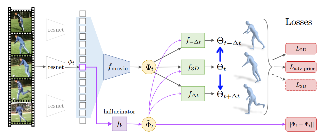
The previous paragraph explains the regressor $f_{3D}$ that maps the movie strip $\Phi_t$ to shape, pose and camera parameters of a human subject. In this section, we will learn more the delta regressors $f_{-\Delta{t}}$ and $f_{\Delta{t}}$ that predict the poses at nearby frames of $-\Delta{t}$ and $\Delta{t}$. In contrast to $f_{3D}$ that predicts both pose and shape, $f_{\Delta{t}}$ just predicts the pose parameters from the movie strip $\Phi_t$.
Specifically, there are two types of delta regressors: past and future regressors
-
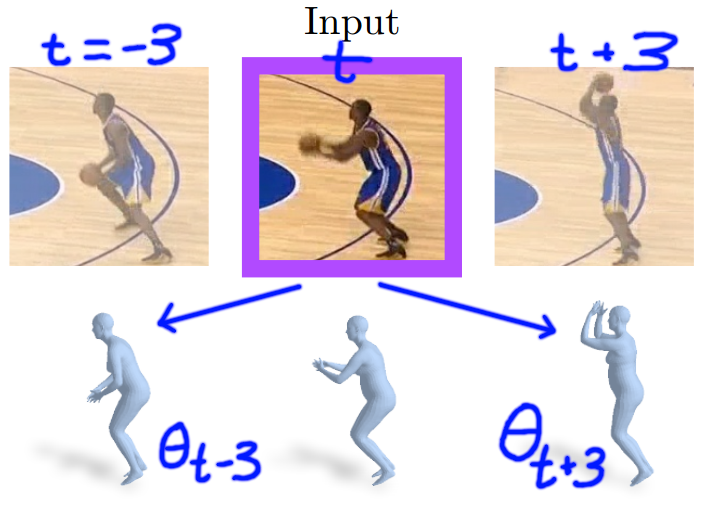
The past regressor $f_{\Delta{t}}$, for example with $\Delta{t} = -3$, predicts pose parameters at frames $(0,1,2)$ from the temporal window features $\Phi$ and pose parameters $\theta$ at frames $(3,4,5)$.
-
The future $f_{\Delta{t}}$, for example with $\Delta{t} = 3$, predicts pose parameters at frames $(3,4,5)$ from the temporal window features $\Phi$ and pose parameters $\theta$ at frames $(0,1,2)$.
These past and future regressors seem counter-intuitive to me at first because it predicts $\theta_{t+\Delta{t}}$, the information that might be already encoded in the input data: the movie strip $\Phi_t$. Why is it necessary to predict an information which is already available in the input? According to the paper, cross-predicting regressors like this help enforce the models to learn temporal cues from frame to frame; therefore, a better 3D dynamics representation (movie strip) $\Phi_t$ will be learned.
Below is a visual example that illustrates the past and future regressors. Given the movie strip $\Phi_t$ that learned, for example, from the temporal window $(t-10, t-9, …,t,…,t+9,t+10)$ and the pose parameters $\theta_t$, the past regressor predicts pose $\theta_{t-3}$, and the future regressor predicts pose $\theta_{t+3}$
Generator-Discriminator mechanism.
We discussed in the previous paragraph that the regressions $f_{3D}$, $f_{-\Delta{t}}$ and $f_{\Delta{t}}$ could predict human shape and pose parameters. However, without a suitable mechanism to constraint their outputs to the human manifold, they will churn out visually displeasing results like in below.
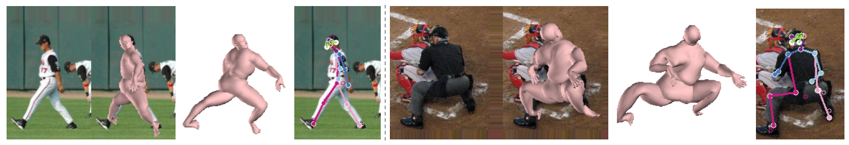
Therefore, different discriminators for shape, single pose joint and the whole joint parameters, are trained to distinguish if these parameters come from generators $f_{3D}$, $f_{-\Delta{t}}$ and $f_{\Delta{t}}$ or the true data in the dataset. In general, the process of training these regressors and the discriminators looks like a competition that both sides get better at their jobs over time. Generators are optimized, through discriminator, in a way that could produce as real as possible parameters. In contrast, discriminator, while being disconnected from the generator, is optimized to classify fake and true parameters.
For more detail about how this mechanism is implemented, please check the paper “End-to-end Recovery of Human Shape and Pose” or my article about this paper.
Dynamics learning losses
In this part, the common losses used for training delta regressors $f_{-\Delta{t}}$ and $f_{\Delta{t}}$ are explained.
3D loss
When the 3D ground truth is available, they could be used to supervise training at 3D levels. There are 3 main types of 3D losses: SMPL shape parameters, SMPL pose parameters, 3D joint locations. The shape and pose parameters are extracted from the predictions, and the 3D joint locations are inferred from the reconstructed SMPL mesh. The code to calculate these losses is shown in below.
The below code shows how the 3D loss function is called. Pose, shape and 3D joints (prediction and ground truth) are passed into the error function. The prediction joints are extracted from the 3D mesh from the SMPL model. For more detail about how this task is implemented, please check the class $OmegasPred$ in the code repository.
loss_e_pose, loss_e_shape, loss_e_joints = compute_loss_e_3d(
    poses_gt=gt.get_poses_rot()[:, s_gt:e_gt],
    poses_pred=pred.get_poses_rot()[:, s_pr:e_pr],
    shapes_gt=gt.get_shapes()[:, s_gt:e_gt],
    shapes_pred=pred.get_shapes()[:, s_pr:e_pr],
    joints_gt=gt.get_joints()[:, s_gt:e_gt],
    # Ignore face pts.
    joints_pred=pred.get_joints()[:, s_pr:e_pr, :14],
    batch_size=(B * seq_length),
    has_gt3d_smpl=has_gt3d_smpl,
    has_gt3d_joints=has_gt3d_jnts,
)
The below code shows how the 3D loss function is implemented. The mean square errors are calculated between pose shape and joints (ground truth vs prediction). For 3D joint losses, before their MSE difference is computed, both ground truth and predictions joints are first translated to their local space by subtracting every joints from their origin, the mid-pelvis point.
def compute_loss_e_3d(poses_gt, poses_pred, shapes_gt, shapes_pred,
                      joints_gt, joints_pred, batch_size, has_gt3d_smpl,
                      has_gt3d_joints):
    poses_gt = tf.reshape(poses_gt, (batch_size, -1))
    poses_pred = tf.reshape(poses_pred, (batch_size, -1))

    shapes_gt = tf.reshape(shapes_gt, (batch_size, -1))
    shapes_pred = tf.reshape(shapes_pred, (batch_size, -1))
    # Make sure joints are B x T x 14 x 3
    assert len(joints_gt.shape) == 4
    # Reshape joints to BT x 14 x 3
    joints_gt = tf.reshape(joints_gt, (-1, joints_gt.shape[2], 3))
    joints_pred = tf.reshape(joints_pred, (-1, joints_pred.shape[2], 3))
    # Now align them by pelvis:
    joints_gt = align_by_pelvis(joints_gt)
    joints_pred = align_by_pelvis(joints_pred)

    loss_e_pose = compute_loss_mse(poses_gt, poses_pred, has_gt3d_smpl)
    loss_e_shape = compute_loss_mse(shapes_gt, shapes_pred, has_gt3d_smpl)
    loss_e_joints = compute_loss_mse(
        joints_gt,
        joints_pred,
        tf.expand_dims(has_gt3d_joints, 1)
    )

    return loss_e_pose, loss_e_shape, loss_e_joints
2D reprojection loss
2D reprojection loss is another MSE error for training the delta regressors. This error is calculated as the MSE between the available ground truth 2D keypoints from the video data and the corresponding reprojected 2D keypoints. In general, the predicted pose $\theta_{t+\Delta{t}}$ will be first transformed to 3D joints through the SMPL model, and then projected to the image plane. The reprojected 2D keypoints will be compared against the ground truth 2D keypoints to calculate reprojection loss. The steps to calculate that loss is shown in below.
Step 1: Calculate the reprojected 2D keypoints from the predicted pose $\theta_{t}$
Step 2: Estimate the optimal scale $s^\star$ and translation $t^\star$ that transforms the reprojected 2D keypoints to match the 2D ground truth keypoints. Specifically, $s^\star$ and $t^\star$ are the solution to the normal equation of the least square error between two keypoint sets.
The simplified code for solving for $s^\star$ and $t^\star$ is shown in below.
# x_vis: visible reprojected 2D keypoints
# x_target_vis: visible ground truth 2D keypoints
# need to compute mean ignoring the non-vis
mu1 = tf.reduce_sum(x_vis, 1, keepdims=True) / num_vis
mu2 = tf.reduce_sum(x_target_vis, 1, keepdims=True) / num_vis
# Need to 0 out the ignore region again
xmu = vis_vec * (x - mu1)
y = vis_vec * (x_target - mu2)

# Add noise on the diagonal to avoid numerical instability
# for taking inv.
eps = 1e-6 * tf.eye(2)
Ainv = tf.matrix_inverse(tf.matmul(xmu, xmu, transpose_a=True) + eps)
B = tf.matmul(xmu, y, transpose_a=True)

scale = tf.expand_dims(tf.trace(tf.matmul(Ainv, B)) / 2., 1)

trans = tf.squeeze(mu2) / scale - tf.squeeze(mu1)
Step 3: Transform the reprojected 2D keypoints from the estimated $s^\star$ and $t^\star$
with tf.name_scope(name, 'batch_orth_proj_idrot', [X, camera]):
    camera = tf.reshape(camera, [-1, 1, 3], name='cam_adj_shape')

    # apply translation t
    X_trans = X[:, :, :2] + camera[:, :, 1:]

    shape = tf.shape(X_trans)
    # apply scale and return
    return tf.reshape(
        camera[:, :, 0] * tf.reshape(X_trans, [shape[0], -1]), shape)
Step 4: Calculate $L_1$ between the transformed reprojected 2D keypoints and ground truth 2D ground truth keypoints.
with tf.name_scope(name, 'loss_e_kp', [kp_gt, kp_pred]):
    kp_gt = tf.reshape(kp_gt, (-1, 3))
    kp_pred = tf.reshape(kp_pred, (-1, 2))

    vis = tf.expand_dims(tf.cast(kp_gt[:, 2], tf.float32), 1)
    res = tf.losses.absolute_difference(kp_gt[:, :2], kp_pred, weights=vis)
    return res
Hallucinator
As defined in the paper, hallucinator is another module that predicts the 3D dynamics representation or movie strip $\Phi_t$ from the feature of a static frame $\phi_t$. As shown in the below code, the design of hallucinator consists of a list of fully connected layers that takes in a single image feature $\phi_t$ and returns a “movie strip” $\Phi_{t}$ - the 3D dynamics representation.
However, from the below code, the input of size of the hallucinator model is actually $T\times 2048$ with $T$ is the temporal sequence length. This seems to be inconsistent with the definition in the paper that the input to the hallucinator is the image feature of a single static image as follows.
def fc2_res(phi, name='fc2_res'):
    """
    Converts pretrained (fixed) resnet features phi into movie strip.

    This applies 2 fc then add it to the orig as residuals.

    Args:
        phi (B x T x 2048): Image feature.
        name (str): Scope.

    Returns:
        Phi (B x T x 2048): Hallucinated movie strip.
    """
    with tf.variable_scope(name, reuse=False):
        net = slim.fully_connected(phi, 2048, scope='fc1')
        net = slim.fully_connected(net, 2048, scope='fc2')
        small_xavier = variance_scaling_initializer(
            factor=.001, mode='FAN_AVG', uniform=True)
        net_final = slim.fully_connected(
            net,
            2048,
            activation_fn=None,
            weights_initializer=small_xavier,
            scope='fc3'
        )
        new_phi = net_final + phi
    return new_phi
The inconsistency also appears at the connection between the hallucinator model and previous stage. For example, the below code passes the extracted image features $self.img_feat_full$ to the hallucinator module, but as shown in the next code, these image features are a concatenation of all image features of a temporal window $(\phi_{t-\Delta{t}}, … ,\phi_t, …,\phi_{t+\Delta{t}} )$, not just the features $\phi_t$ of the center frame. I will drop an email to the authors to clarify this point.
if self.do_hallucinate:
    # Call the hallucinator.
    pred_phi = self.img_feat_full
    # Take B x T x 2048, outputs list of [B x T x 2048]
    self.pred_movie_strip = self.f_hal(pred_phi)
The calculation of self.img_feat_full is shown in below.
print('Getting all image features...')
# Load all images at once. I_t should be B x T x H x W x C
I_t = self.image_loader[:, :]
# Need to reshape I_t because the input to self.f_image_enc needs
# to be B*T x H x W x C.
I_t = tf.reshape(I_t, (self.batch_size * self.sequence_length,
                       self.img_size, self.img_size, 3))
img_feat, phi_var_scope = self.f_image_enc(
    I_t, weight_decay=self.e_wd, reuse=tf.AUTO_REUSE)
self.img_feat_full = tf.reshape(
    img_feat, (self.batch_size, self.sequence_length, -1))
Conclusion
In this article, I summarized the main ideas of the paper “Learning 3D Human Dynamics from Video” that learns the 3D dynamics of a human subject from a set of temporal sequence of images. According to the author, learning from a temporal sequence will help stabilize the quality of the resulting mesh. It also opens the chance to learn a new model called hallucinator that predicts next movements from the a single static image. Unfortunate, this modules seem still unavailable from the test code the author’s repository. For further question, please contact me through my email.