SMPL Human Model Introduction
This article could be served as a bridge between the SMPL paper and a numpy-based code that synthesizes a new human mesh instance from a pre-trained SMPL model provided by the Maxplank Institute. I wrote it as an exercise to strengthen my knowledge about the implementation of the SMPL model.
Introduction
3D objects are often represented by vertices and triangles that encodes their 3D shape. The more detail an object is, the more vertices it is required. However, for objects like human, the 3D mesh representation could be compressed down to a lower dimensional space whose axes are like their height, fatness, bust circumference, belly size, pose etc. This representation is often smaller and more meaningful.
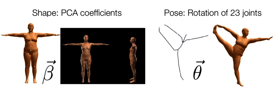
The SMPL is a statistical model that encodes the human subjects with two types of parameters:
-
Shape parameter: a shape vector of 10 scalar values, each of which could be interpreted as an amount of expansion/shrink of a human subject along some direction such as taller or shorter.
-
Pose parameter: a pose vector of 24x3 scalar values that keeps the relative rotations of joints with respective to their parameters. Each rotation is encoded as a arbitrary 3D vector in axis-angle rotation representation.
 the image is taken from the SMPL paper
As an example, the below code samples a random human subject with shape and pose parameters. The shift and multiplication are applied to bring the random values to the normal parameter range of the SMPL model; otherwise, the synthesized mesh will look like an alien.
pose = (np.random.rand((24, 3)) - 0.5)
beta = (np.random.rand((10,)) - 0.5) * 2.5
Human synthesis pipeline
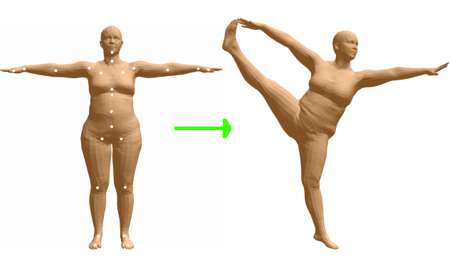
The process of synthesizing a new human instance from the SMPL model consists of 3 stages as illustrated in the below figure.
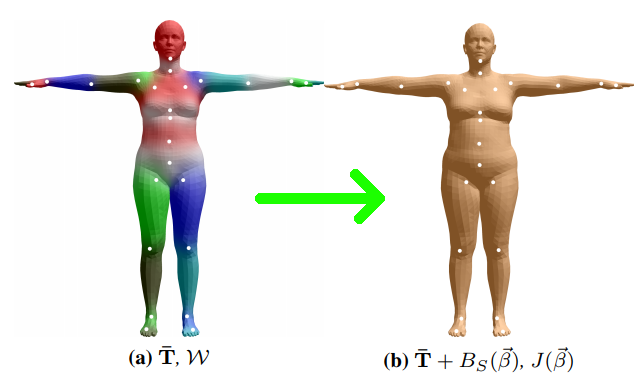
- Shape Blend Shapes: In this step, a template(or mean) mesh $\bar{T}$ is added with vertex displacements that represent how far the subject shape is from the mean shape.
 The image is taken from the SMPL paper
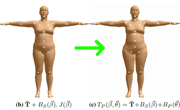
- Pose Blend Shapes: After the identity mesh is constructed in the rest pose, it is further added with vertex displacements that explain for deformation correction caused by a specific pose. In other words, the pose in the next step “Skinning” results in some amount of deformation on the rest pose at this step.
 The image is taken from the SMPL paper
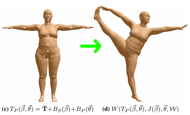
- Skinning: Each mesh vertex from the previous step is transformed by a weighted-combination of joint deformation. To put it simply, the closer to a vertex a joint is, the stronger the joint rotates/transforms the vertex.
 The image is taken from the SMPL paper
Shape Blend Shapes
The rest pose shape is formed by adding the mean shape with a linear combination of principal shape components (or vertex deviations), which denote the principal changes among all the meshes in the dataset. Specifically, each principal component is a $6890\text{x}3$ matrix, which represent $(x,y,z)$ vertex displacements from the corresponding vertices of the mean mesh. To make it more clear, below is a visualization of the first and second principal components of the SMPL model. The mesh pair for each component is constructed adding/subtract the component to/from the mean mesh an amount of 3 standard deviations ,as showned in the below equation:
From the visualization, it seems that the first component explains for the change in height and the second represents the change in weight among human meshes.
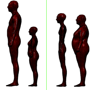
the image is taken from the Maxplank Institute
The below code creates a new mesh by linearly combining 10 principal components from the SMPL model. The more principal components we use, the less the reconstruction error is; however, the SMPL model from the Maxplank Institute just provides us with the first 10 components.
# shapedirs:  6890x3x10:  10 principal deviations
# beta:       10x1:       the shape vector of a particular human subject
# template:   6890x3:     the average mesh from the dataset
# v_shape:    6890x3:     the shape in vertex format corresponding to the shape vector
v_shaped = self.shapedirs.dot(self.beta) + self.v_template
Pose Blend Shapes
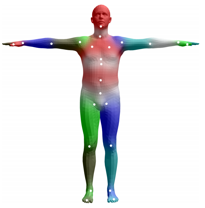
In the SMPL model, the human skeleton is described by a hierarchy of 24 joints as shown by the white dots in the below figure. This hierarchy is defined by a kinematic tree that keeps the parent relation for each joint.
 The image is taken from the SMPL paper
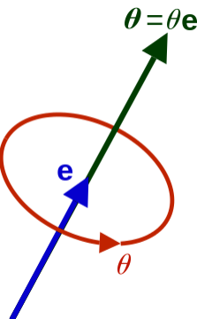
The 24-joints hierarchy is represented by $(23\text{x}3)$ matrix corresponding to $23$ relative rotations from parent joints. Each rotation is encoded by a axis-angle rotation representation of $3$ scalar values, which is denoted by the $\boldsymbol{\theta}$ vector in the below figure.
The image is taken from the Wikipedia
The relative rotations of 23 joints $(23\text{x}3)$ causes deformation to surrounding vertices. These deformations are captured by a matrix of (23x6890x3) which represents $23$ principal components of vertex displacements of $(6890x3)$. Therefore, given a new pose vector of relative rotation 23x3x3 values as weights, the final deformation will be calculated as a linear combination of these principal components.
# self.pose :   24x3    the pose parameter of the human subject
# self.R    :   24x3x3  the rotation matrices calculated from the pose parameter
pose_cube = self.pose.reshape((-1, 1, 3))
self.R = self.rodrigues(pose_cube)

# I_cube    :   23x3x3  the rotation matrices of the rest pose
# lrotmin   :   207x1   the relative rotation values between the current pose and the rest pose
I_cube = np.broadcast_to(
      np.expand_dims(np.eye(3), axis=0),
      (self.R.shape[0]-1, 3, 3)
    )
lrotmin = (self.R[1:] - I_cube).ravel()

# v_posed   :   6890x3  the blended deformation calculated from the
v_posed = v_shaped + self.posedirs.dot(lrotmin)
Skinning
 The image is taken from the SMPL paper
In this step, vertex in the rest pose are transformed by a weighted combination of global joint transformations (rotation + translation). The joint rotations are already calculated from the pose parameter of the human subject, but the joint translation part needs to be estimated from the corresponding rest-pose mesh of the subject.
Joint Locations Estimation
Thanks to the fixed mesh topology of the SMPL model, each joint location could be estimated as an average of surrounding vertices. This average is represented by a joint regression matrix learned from the data-set that defines a sparse set of vertex weight for each joint. As shown in the below figure, the knee joint will be calculated as a linear combination of red vertices, each with a different weight.
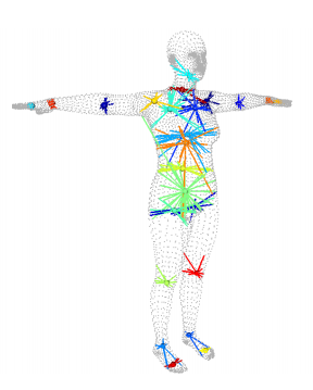
The image is taken from the SMPL paper
The below code shows how to regress joint locations from the rest-pose mesh.
# v_shape:          6890x3    the mesh in neutral T-pose calculated from a shape parameter of 10 scalar values.
# self.J_regressor: 24x6890   the regression matrix that maps 6890 vertex to 24 joint locations
# self.J:           24x3      24 joint (x,y,z) locations
self.J = self.J_regressor.dot(v_shaped)
Skinning deformation
The joint transformations cause the neighboring vertices transform with the same transformations but with different influence. The further from a joint a vertex is, the less it is affected by the joint transformation. Therefore, a final vertex could be calculated as a weighted average of its versions transformed by 24 joints.
The below code first calculates the global transformation for each joint by recursively concatenating its local matrix with its parent matrix. These global transformations are then subtracted from the corresponding transformations of the joints in the rest pose. For each vertex, its final transformation is calculated by blending the 24 global transformations with different weights. The code for these steps are shown in the below.
# world transformation of each joint
G = np.empty((self.kintree_table.shape[1], 4, 4))
# the root transformation: rotation | the root joint location
G[0] = self.with_zeros(np.hstack((self.R[0], self.J[0, :].reshape([3, 1]))))
# recursively chain transformations
for i in range(1, self.kintree_table.shape[1]):
  G[i] = G[self.parent[i]].dot(
    self.with_zeros(
      np.hstack(
        [self.R[i],((self.J[i, :]-self.J[self.parent[i],:]).reshape([3,1]))]
      )
    )
  )

# remove the transformation due to the rest pose
G = G - self.pack(
  np.matmul(
    G,
    np.hstack([self.J, np.zeros([24, 1])]).reshape([24, 4, 1])
    )
  )
# G       : (24, 4, 4)  : the global joint transformations with rest transformations removed
# weights : (6890, 24)  : the transformation weights for each joint
# T       : (6890, 4, 4): the final transformation for each joint
T = np.tensordot(self.weights, G, axes=[[1], [0]])

# apply transformation to each vertex
rest_shape_h = np.hstack((v_posed, np.ones([v_posed.shape[0], 1])))
v = np.matmul(T, rest_shape_h.reshape([-1, 4, 1])).reshape([-1, 4])[:, :3]

# add with one global translation
verts = v + self.trans.reshape([1, 3])
Conclusion
In this port, we went through the steps of synthesizing a new human subject from the trained SMPL model provided by the Maxplank institute. We learned how to combine principal shape components to reconstruct the rest-pose shape and then regress the joint locations from it. We also learned to predict the deformation correction caused by pose and apply global joint transformation to the rest-pose mesh. For further information, please check the SMPL paper